Introduction
Estuaries are transition zones between land and sea and are important to aquatic organisms. (Levin et al. 2001). They are increasingly under threat from anthropogenic influence the world over. The size, shape and volume of water distinguish one estuary from another and these features are greatly influenced by the geofraphical landscape of the region. However estuaries have certain common features, such as gradients in their salinity and sediments which are known to influence the biological communities found within the systems.
Estuaries are among the most productive natural habitats on earth due to sea and fresh water inflow that adds nutrients to the water column and sediment. This makes them highly productive and enables them to support large diversity of aquatic organisms. Intertidal,macrobenthos are found between high and low tide marks, either permanently living on or within soft sediments. These organisms are of ecological importance and are mainly used as indicator species within these habitats. Faunal distribution within the estuary is determined greatly by salinity, temperature, organic matter, concentration of oxygen and composition of sediments.
Primary productivity, competition and adaptation to the estuarine climate also influence the temporal and spatial and temporal differences in benthic species composition. However, the composition of the fuana present at a given estuary are a clear indicator of the state of the aquatic environment (Warwick & Ruswahyuni, 1987). Salinity and sedimentation are however the two major challenges faced by organisms living within the estuaries. Bacteria; most of which have high oxygen demand are found in abundance within the sediment hence reduce the amount of oxygen in these zones (Elliott, 2004).
Aim of the study
The major aim of the study was to examine the influence of the major gradients in physical factors (salinity and sediments) on the distribution of benthic organisms within the Waiwera Estuary.
Literature review
Macrobenthic invertebrates are important components of estuarine ecosystems, in terms of productivity. They provide an important food source for other organisms which depend on these eshtuaries for survival. (Herman et al., 1999). “Estuarine organisms can be described as bioindicators in three ways, as: 1) indicators of a defined set of environmental conditions; 2) indicators of contaminant loads on the system; and 3) indicators of the overall health of the system” (Wilson, 1994).
The assemblage of macrobenthos along estuarine salinity gradient are classified into polyhaline, mesohaline and oligohaline zones corresponding to marine , brakish water and fresh water respectively. (Giberto et al., 2007). However the species within these zones are not permanent due to spatial and temporal fluctuations in environmental conditions along these areas. (Ysebaert et al., 1998). Studies by Sanders et al., 1965 found that salinities in the interstices are more stable and different from those of the water column and hence organisms living in these interstices are not always directly affected by salinity changes (Sanders et al. 1965).
The variation in salinity both vertically and horizontally are the determinants of salinity structure within the estuaries. Its distribution within an estuary is a reflection of the relative influx of fresh water andn marine water. The ocean currents and wind aid in mixing of marine and fresh water. Most aquatic macrobenthos function properly at optimum salinity levels below or above which they may lose their ability for osmoregulation. Consequently, the distribution of macrobenthos can be affected by shifting salinity distributions. Few species are usually characteristic of estuaries with wide ranging morphological and physico-chemical parameters (Kanandjembo et al., 2001). For instance, while bivalves and gastropods are affected by sediment characteristics, polychaetes and amphipods do not (Wu and Shin, 1997).
Dissolved oxygen (DO) is the amount of oxygen dissolved in water and it is meassured in mg/l O2 . It is slightly soluble in water ranging between 6 to 14 mg/l. However, its solubility varies inversely with salinity, temperature and pressure. D.O defines the type of organisms that are most likely to be found in a given water body and it’s concentration varies diurnally due to tidal exchange (Connel and Miller, 1984; Best et al., 2007). Estuarine health and balance can be assessed by its biodiversity levels.
The densities of some organisms may be high in some parts of an estuary, however this should not be taken as an indicator of a productive habibtat since it may just be a reflection of the adaptability of that particular organism to that specific habitat. Sedimentation refer to the amount of organic and mineral material deposited on the bottom of a water body over a given period of time. It is measured in terms of sediment density per unit area over a given time period or as vertical accumulation over time. Macrobenthos are mostly controlled by the nature of sediment present on the sea floor and the dissolved oxygen status at the bottom of the water bottom of the water body.
Study site description
The study was carried out along Waiwera estuary situated about 35 km North of Auckland on the Eastern coast (Fig. 1). Two major streams, the Waiwera and the Wainui form the Waiwera Estuary. The drainage area is a steep slope covering an area of approximately 500-600 ha of pastoral agricultural land and bush. The Waiwera estuary is a relatively small tideway, which extends only 3.5 km inland. It is well flushed with tidal velocities of up to 0.50 m s-l.
At mean high tide there is about 1.5-2 m of water covering the shore while at low tide the water flow is restricted to a single 20 m wide by 1-1.5 m deep river channel, leaving extensive tidal flats throughout large parts of the estuary. The drainage basin receives an annual rainfall of between 1250-1400 mm with the lowest monthly precipitation occurring during the month of February and the highest in August and September. The sediment consists of a mixture of dead shells, sand and silt.

Materials and Methods
Benthic organisms inhabiting the sediment habitat were selected for this study as most of them are bottom dwellers and are known to occupy specific niches on the floor of the sea therefore serving as a reflection of the state of the estuary. A total of eight stations along the estuary spreading from the mouth of the estuary up to nearly the extent of tidal influence- a distance of approximately five kilometers were sampled. Students were divided into equal teams of 4-6 individuals and each team sampled one to three stations along the estuary.
Samples were collected at three tidal levels (lower, middle and upper shores) at each station. In areas that had mangroves, the upper level was taken as the inner part of the mangrove forest, the middle level as the seaward edge of the mangrove forest and the lower level as the edge of the tidal channel. Sampling was only done in areas that had thick layers of sediment while areas with emergent rocks and compacted mud (plastic or clay-like) were avoided. During sampling, great care was taken to avoid trampling the emergent pneumatophores and seedlings of mangrove plants.
Using a 0.1m2 quadrant, a total of five 0.1 m2 samples were collected using a trowel to depths of 15cm at each station and sieved using a 3 mm mesh size sieve. One sediment sample scooped by half a trowel full down to 5cm depth was collected also collected and placed in a plastic bag labeled using a marker pen. The sediment sample was later dried and sieved into major fractions to determine the particulate composition.
For each replicate sample, organisms were removed from the mesh, identified, counted and recorded on the datasheet. Seaweeds, mangrove pneumatophores, seedlings and seeds were also included. Unidentified specimens were placed in separate; carefully labeled jars for later matching and identification of species. The unidentified species were recorded appropriately in a data sheet for later identification. A representative range of specimen from each site were then put into a plastic bag so that at the end of the day, all the other groups could see what organisms were at the stations they didn’t sample.
At each level the presence of burrow openings, casts, trails of organisms on the surface and profile (from the intact side of the hole where sampling was done) were recorded. The colour of sediments on the surface and down the subsurface profile were also recorded (since the depth of the anoxic layer was of great interest in the study). Identification of organisms was done using an illustrated guide to common macroinvertebrates species. Data on the water column depth measured using Hummingbird handheld depth sounder, and salinity and temperature, measured using a YSI probe at each site from a small boat in 2002 was provided. The present station numbers were matched with the ones sampled initially in 2002. However, some new stations were sampled in this study while others were ignored or extrapolated as appropriate from those sampled in 2002.
Study Findings: Environmental Parameters
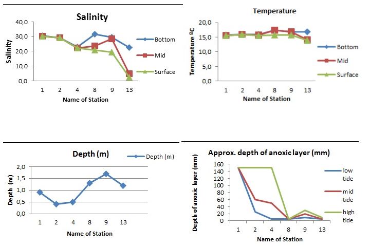
Salinity in the Waiwera estuary remained considerably high throughout five stations while station the sixth (station 13) had relatively low salinity (below 5ppt) for high and mid tide while the low tide was slightly higher. Station 8 displayed a strong variation between the low, mid and high tides at 31, 24 and 21 ppt respectively whereas there was no significant variations in salinity between the three different regions for station 1, 2 and 4. However, there were slight variations in salinities between the stations. Salinity values were almost similar for low and mid tide for station 9 but showed a higher value for the high tide.( Fig 2A)
Temperatures were mostly constatnt (btw 15-160C) in three stations (1, 2 & 4) and among the different tide levels whereas it showed a slight variation in temperature with high and mid tide recording 140C each while high tide recorded 16.50C. (Fig 2B).
The six stations varied greatly in terms of depth with station 9 being the deepest at 1.7m and station 2 the shallowest at 0.4m. Stations 1, 4, 8 & 13 were 0.9m, 0.5m, 1.3m and 1.2m respectively.The approximate depth of annoxic layer (mm) was extremely low in stations 8 and 13 but high in station 1. Stations 2 and 4 showed a significant variation especialyy in the low, mid and high tides.(Fig 2C) The wide variation between high and low tide was clear in station 4 (at about 5mm annoxic depth for lowtide and 140mm for high tide).The depth of the anoxic layer was highest in the three tide levels of station one. This station showed significantly higher depths of anoxic layer and interesting the trend was the same for all the tide levels (low, mid and high tides). Station two and four had significant variations between low, mid and high tide levels. Station 8 and 13 however had extremely low depths of anoxic layer in the three tide levels (Fig 2D).
Sediment composition
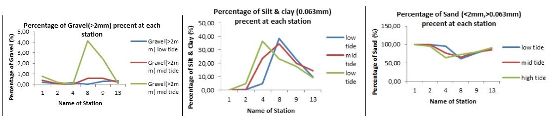
All the six stations sampled had just a small percentage (less than 1%) of gravel above 2mm in size in the low and mid and some high tide. The high tide of station 8 and 9 however had 4.5% and 3% gravel of <2mm respectively (Fig. 3A). Silt and clay on the other hand varied significantly between the six stations. Whereas stations 1 and 2 had silt and clay percentages of less than 10, stations 4, 8 & 9 were relatively high ranging between (20-40%).
Percentage silt in station 13 for low, mid and high tide were slightly higher. (Fig 3B). this was a clear indication of the variability of sediment composition between the six stations sampled along Wawira estuary. Generally, all stations had high percentages of silt as compared to other sediment types. Station 1 and 2 comprised of about 100% sand in all the three tide levels while station 4 had asignificant variation between the high, mid & low tide in terms of percentage composition of sand, whereby high, tide had 60%, mid tide 70% and low tide 90%.(Fig. 3C).
Diversity, abundance and distribution
A maximum of 26 species were recorded across the six stations that were sampled.(Fig. 4). The most abundant specie was Austrovenus stutchbury (Cockle) which had the largest number of individuals in low and mid tide. However, this specie was completely absent in the high tide probably because of the harsh conditions at this site which inhibited their survival. Paphies australis (pipi) and Helice crassa and F. nereididae (tunneling and mud crab) also occured in significant quantities within the estuary. Only two species F nereididae and Helice crassa (tunnelling mud crab) occured across all the tide levels though in relatively smalller numbers.
Other species which occured within the estuary albeit in smaller numbers in the low, mid and high tide included, zeacumantus lutucentus (mud flat hornshell) which was present in low and high tide and absent in mid tide., Cominella glandiformis (whelk), Macomona liliana (wedge shell), Diloma subrostrata (mud flat topshell) and Nucula hartvigiana (nut shell). F corophiidae and potamopyrgus estuarinus (snail) only occured in the high tide though in small numbers. Talorchestia quoyana (sand hoppers), F paguridae (hermit crab), Pyromaia tuberculata (crab) occured in very low numbers and were completely absent in the three different habitats. Chiton glaucus (green chiton) was only found in the low tide but in very low numbers. In general, a relatively large number of species inhabited the low tide region (14 spp) as compared to mid tide (12 spp) and high tide (6 spp).
Discussion
The change in faunal abundance was roughly linked to changes in sediment characteristics within the Waiwera Estuary. On the low tide, the influence of wave action is considered to be the major factor affecting the fauna as it results in a decrease in evenness and species richness; on the other hand, muddy substratum were found to decrease the density of fauna. The highest species diversity was found on the silty and sand substratum. There is therefore a close correlation between the sediment size and the abundance of fauna.In an estuary there is a clear gradient of water salinity from the seaward to the upstream area due to river water inflow.
However, the salinity profile of the water changes over time as the result of tidal action, meteorological influences and wind. Estuarine organisms must tolerate such strong and variable environmental stresses. In general, the diversity of aquatic organisms tends to be limited in estuaries due to the relatively severe environmental conditions. Benthic species also have a response to changes in fresh water inflow. Under high inflow, macrobenthic organisms adapted to low salinities flourish until higher salinity conditions return. The more marine species reappear and rebuild to higher levels that existed before the high inflow conditions commenced In conclusion, the high density of macrobenthos are considered to be related to relatively stable conditions.
References
Best, A. A., Wither, A. W. and Coates, S. (2007). Dissolved oxygen as a physico-chemical supporting element in the water framework directive. Marine Pollution Bulletin 55, 53-64.
Connell, D. W. and Miller, G. J. (1984). Chemistry and Ecotoxicology of Pollution. John Wiley & Sons, N.Y.
Elliott, M. (2004) The Estuarine Ecosystem: ecology, threats and management. New York: Oxford University Press Inc. Web.
Giberto, D. A., Bremec, C. S., Cortelezzi, A., Rodrigues Capitulo, A. and Brazeiro, A. (2007). Ecological boundaries in estuaries: macrobenthic beta-diversity in the Rio de la Plata system (34-36oS). Journal of the Marine Biological Association U.K. 87: 377-381.
Herman, P. M. J., Middleberg, J. J., Van De Koppel, J. and Heip, C. H. R. (1999). Ecology of marine macrobenthos. Advances in Ecological Research. 29: 195-240.
Kanandjembo, A. N., Platell, M. E. and Potter, I. C. (2001). The benthic macroinvertebrate community of the upper reaches of an Australian estuary that undergoes marked seasonal changes in hydrology. Hydrological Processes 15: 2481-2501.
Levin, L. A., Boesch, D. F., Covich, A., et al. (2001). The function of marine critical transition zones and the importance of sediment biodiversity. Ecosystems 4: 430-451.
Sanders, H. L., Mangelsdorf, P. C. and Hampson, G. R. (1965). Salinity and faunal distribution in the Pocasset River, Massachusets. Limnology and Oceanography 10: R216-R229.
Warwick, R. M. and Ruswahyuni, K. (1987). Comparative study of the structure of some tropical and temperate marine soft-bottom macrobenthic communities. Marine Biology. 95: 641-649.
Wilson, J. G. (1994). The role of bioindicators in estuarine management. Estuaries 17: 94-101.
Wu, R. S. S. and Shin, P. K. S. (1997). Sediment characteristics and colonization of soft-bottom benthos: a field manipulation experiment. Marine Biology 128: 475-487.
Ysebaert, T., Meire, P., Coosen, J. and Essink, K. (1998). Zonation of intertidal macrobenthos in the estuaries of Schelde and Ems. Aquatic Ecology 32: 53-71.