Abstract
This research report discusses about the impact of age, department, tenure, gender and position on the samples drawn. The gender disparity and its impact on the job satisfaction, how male and female get satisfied with their job. This particular issue was deemed relevant due to its depth and impact on virtually all aspects of an organization.
Introduction
A survey was conducted to determine the influence of gender, position, age, department and tenure on job satisfaction. The survey consisted of similar questions on job satisfaction with response options. The participant answered by selecting a value on a seven-point scale.
The answers are marked and merged, through a excel, into a personality profile which represents how strongly each of the basic desires features. This was handled anonymously. The results are presented in an easy to use graphics along with a comprehensive assessment report.
The scales were formed by adding the values of the individual questions of the scales by giving equal weight to each question. All categorical items on workload and strain were transformed on a value range from 1 (least satisfied) to 7 (most satisfied). In this case, the questions had seven response options with value of 1, 2, 3, 4, 5, 6 and 7.
The scale value is computed as the simple average. Answer refusals or participants that answered less than half of the questions are considered missing. For the participants that answered at least half, the scale value was computed as the average of the answered questions.
Chosen Variables
The variables chosen were gender for qualitative variable and Extrinsic for your quantitative variable.
Difference in variable types
A qualitative variable sometimes-called predictor variable. It is varied and manipulated by a researcher. It is referred to as presumed cause of an event.
It determines the value of other variables. It is manipulated to create an effect on other variable (Bhattacharya and Johnson, 1997).). Quantitative variables are the variables, which a researcher/experimenter measures after altering other variables which affect quantitative variable (Wierenga & Bruggen, 1998).
This case is sufficient to understand the significance of both the quantitative and qualitative variables in a quantitative research methodology. The values of qualitative variables are derived from quantitative variables which can be altered further by variation the values of quantitative variables(Healy, 2009).
Qualitative variable is considered as presumed cause of an event where as a quantitative variable is considered as the presumed effect of an event. The major difference between an qualitative and a quantitative variable is that quantitative values of qualitative variable can be altered by changing the values of the qualitative variable. It means that the values of qualitative variable are constant while those of quantitative variables are prior to changes (Babbie, 2009).
Descriptive statistics: Qualitative variable
Explanation of descriptive statistics
From the table above, it could be suggested that the standard deviations are close to the mean value of the variable. The reason for using gender is that on two options either 1 of two. The standard deviations are 0.4837 on either side of the mean.
Furthermore, by observing the values of the variable collected 72 participants it could be concluded that the data is normally distributed as majority of the values lie within two standard deviations of the mean value. This is further proved by comparing the mean, median and mode values obtained in the table. The mode and mode are 1.
Descriptive statistics: Quantitative variable
Explanation of descriptive statistics
Table above showed that statistical data derived using the excel program. Based on the statistical data, the mean was 5.45 with a standard deviation value of 0.4299. From this table, it could be inferred that mean, median and mode values are very close to each other, which is supportive of the normal distribution of data. The table presents an approximate normal distribution and showed homogeneity of variance.
If these amounts were arranged on a graph, the frequency distribution would reflect the process variability. The values would be clustered close to the process average, but some of the values would vary somewhat from the mean. They too would have a distribution of values.
Chart/Graph for qualitative variable

Description of Chart
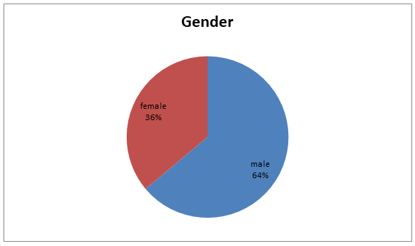
Looking at the gender of the respondents it indicates that 26 were females and 46 were males this represents 36% and 64% of females and males respectively.
Chart/Graph for quantitative variable

Description of Chart
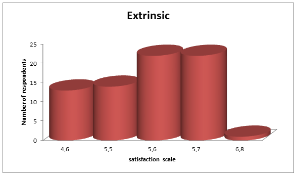
The chart shows that 5.6 and 5.7 scales had 22 respondents each while 4.6 and 5.5 had 14 and 13 respectively, only one had 6.8 score.
Explanation of standard deviation and variance
Standard deviation is the variations from the mean while variance square of the standard deviations. The standard deviation shows that the data has a greatest deviation from the mean. What it means that the mean is widely dispersed that’s why it has a larger standard deviation.
This reflects the averaging that occurs in computing the sample means: high and low values in samples tend to offset each other, resulting in less variability among sample means than among individuals’ values. Note that both distributions have the same mean; the mean of the sampling distribution is exactly equal to the mean of the process.
Finally, note that the sampling distribution is normal distribution, even if the process distribution isn’t normal. The central limit theorem provides the basis for the assumption that the sampling distribution will be normal or at least approximately normal, even if the population is not.
The normal distribution can be used to help judge whether a process is performing adequately. If the output reflects only random variability, one would conclude that the process is stable. However, if there were evidence of nonrandom variability, one would conclude that the process is unstable.
Importance of charts and graphs
In a charts and graph shows how the variable are distributed. They are pictorial representation of the results of the company. The finding through the diagram is further reinforced by the value of the tables between the variables under consideration.
Conclusion
From the results analysis above, it can be concluded most people interviewed are satisfied. The present study also dissuades any conception about the differences between male and female in job satisfaction. The study treats both genders at par.
However, there are traditional arguments suggesting that males tend to be more aggressive and dominating, and demanding as well as have stakes in major decision-making processes. Whereas, females behave in a submissive manner and do not have bargaining power comparing to male counterparts. These are not considered and invalidated as out of scope for this particular study.
References
Babbie, E. R. (2009). The basics of Social Research. Belmont, CA: Cengage Learning.
Bhattacharya, G., & Johnson, R. (1997). Statistical Concepts and Methods. New York: John Wley & Sons.
Healy, J. F. (2009). Statics: A Tool for Social Research. Belmont, CA: Cengage Learning.
Wierenga, B., & Bruggen, G. V. (1998). The Dependent Variable In Research Into Effects of Creativity Support System: Quality and Quantity of Ideas. M I S Quarterly , 81-87.