A-Level Math AQA : Specification Presentation

What is AQA?

Assessment and Qualifications Alliance (AQA) is an independent charitable organisation that produces specifications and examination assignments for 12th and 13th-grade students studying various A-Level disciplines, including mathematics.

In order to maintain relevance and improve the efficiency of education, the AQA is continuously modifying the programmes created. Thus, the specifications described in this project have an expiry date of two years, starting from 2018.

Motivation for Selecting a Specification

For educational institutions, students, and private teachers, the choice of AQA is based on:

1. relevant specification;
2. cooperation with many universities;
3. compliance with the requirements of the Department for Education for A-Level mathematics studies;
4. excellent assessment structure based on multifactoriality and universality of knowledge;
5. proposed incentive policy.

Teaching Aids for Studying

Route Maps [All About Maths] — this book is designed for teachers who develop their methodological plans based on the AQA specification.

Teaching Guide [All About Maths] — this is another teacher’s manual, which distinguishes between the levels of specification, provides assessment criteria and supports teachers in finding new materials.

Textbooks — the textbook collection.

Command words — this website describes the terms used to design the examination questions.

Materials for Preparing for the Exam

Assessment resources — this web page contains a list of numerous publications, manuals, PDF documents and text files that describe strategies for designing examination tasks, answer evaluation methodologies and sample tasks.

The Additional Benefit

A considerable advantage of using AQA as a guiding specification for the design of a mathematics course is the availability of an online tool for evaluating the results achieved by students.

Enhanced Results Analysis, ERA is an excellent tool that offers a platform for comparing academic results with past or other students and other schools. By using the ERA, the teacher decides whether to compare academic performance, develop an individual learning plan, or address the weaknesses of individual students.

Course Structure

The essential principles of the developed course on AQA specifications:

1. the study of disciplines is based on a linear mechanism: students will be able to test their knowledge through examinations traditionally taken at the end of the course.
2. The specifications require the student to use the full range of knowledge and skills discussed in OT1-OT3 (discussed later) to demonstrate problem-solving skills and answer questions in sections A-S (discussed later).
3. There are three scenarios underlying the modelling of the exam. In total, three works can give a student 300 points.

Course Objectives

The purpose of the specifications is to reward the following academic qualities of a student:

• confident knowledge of the mathematical apparatus;
• expansion of thematic skills and abilities;
• a comprehensive understanding of interrelated topics;
• use of mathematics in other areas of knowledge;
• logical thinking skills;
• building the evidence base;
• identifying cases where the task at hand justifies the use of mathematics;
• modelling charts and graphs;
• interpretation of conclusions and creation of conclusions.

Evaluation Objectives

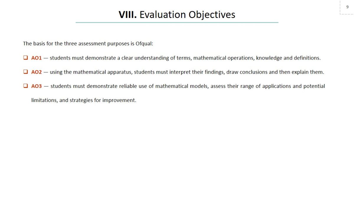
The basis for the three assessment purposes is Ofqual:

• AO1 — students must demonstrate a clear understanding of terms, mathematical operations, knowledge and definitions.
• AO2 — using the mathematical apparatus, students must interpret their findings, draw conclusions and then explain them.
• AO3 — students must demonstrate reliable use of mathematical models, assess their range of applications and potential limitations, and strategies for improvement.

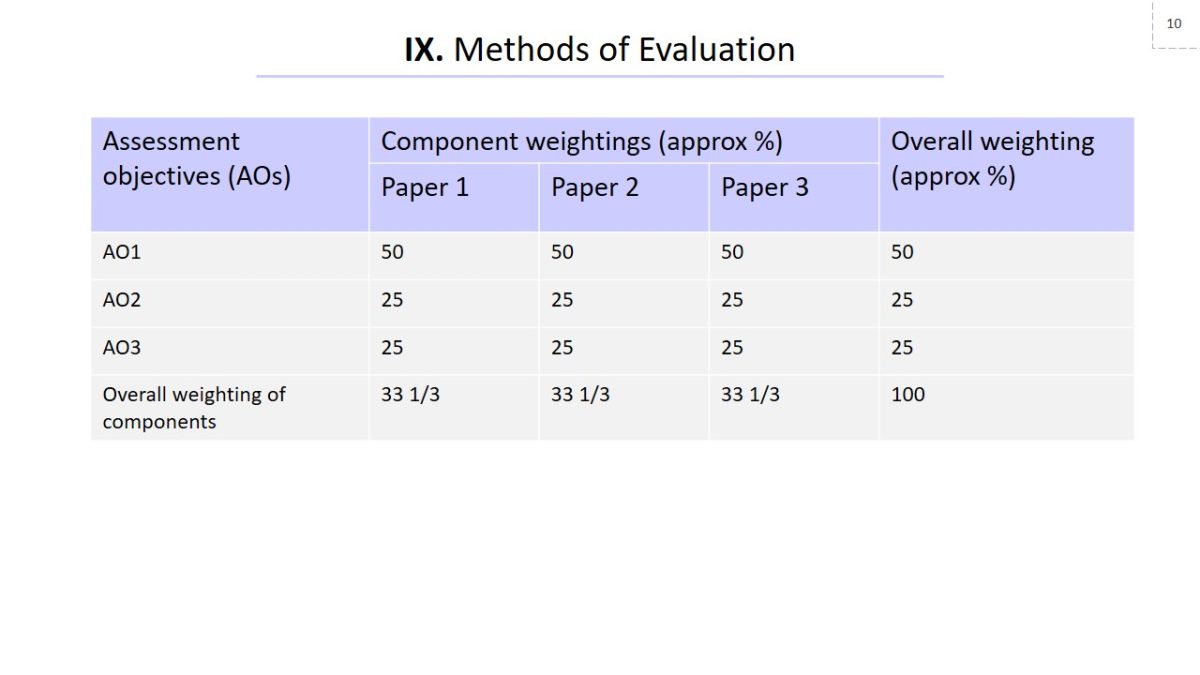
Methods of Evaluation

Points Failure

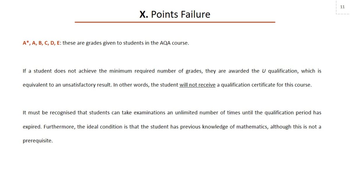
A*, A, B, C, D, E: these are grades given to students in the AQA course.

If a student does not achieve the minimum required number of grades, they are awarded the U qualification, which is equivalent to an unsatisfactory result. In other words, the student will not receive a qualification certificate for this course.

It must be recognised that students can take examinations an unlimited number of times until the qualification period has expired. Furthermore, the ideal condition is that the student has previous knowledge of mathematics, although this is not a prerequisite.

Additional Conditions

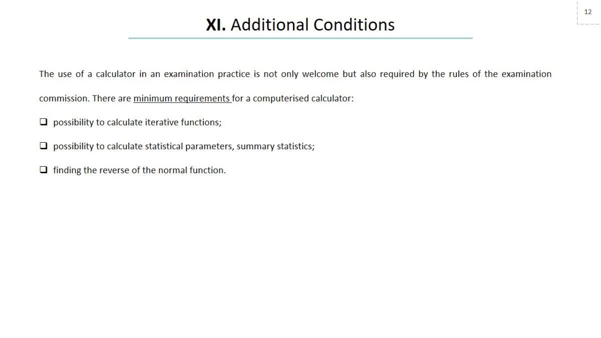
The use of a calculator in an examination practice is not only welcome but also required by the rules of the examination commission. There are minimum requirements for a computerised calculator:

• possibility to calculate iterative functions;
• possibility to calculate statistical parameters, summary statistics;
• finding the reverse of the normal function.

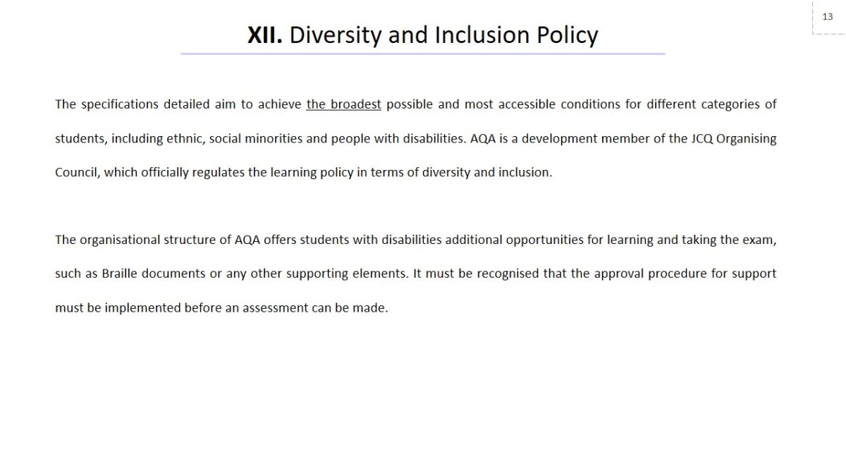
Diversity and Inclusion Policy

The specifications detailed aim to achieve the broadest possible and most accessible conditions for different categories of students, including ethnic, social minorities and people with disabilities. AQA is a development member of the JCQ Organising Council, which officially regulates the learning policy in terms of diversity and inclusion.

The organisational structure of AQA offers students with disabilities additional opportunities for learning and taking the exam, such as Braille documents or any other supporting elements. It must be recognised that the approval procedure for support must be implemented before an assessment can be made.

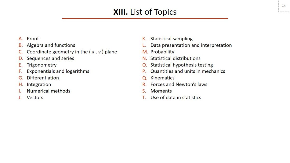
List of Topics

1. Proof;
2. Algebra and functions;
3. Coordinate geometry in the ( x , y ) plane;
4. Sequences and series;
5. Trigonometry;
6. Exponentials and logarithms;
7. Differentiation;
8. Integration;
9. Numerical methods;
10. Vectors;
11. Statistical sampling;
12. Data presentation and interpretation;
13. Probability;
14. Statistical distributions;
15. Statistical hypothesis testing;
16. Quantities and units in mechanics;
17. Kinematics;
18. Forces and Newton’s laws;
19. Moments;
20. Use of data in statistics.

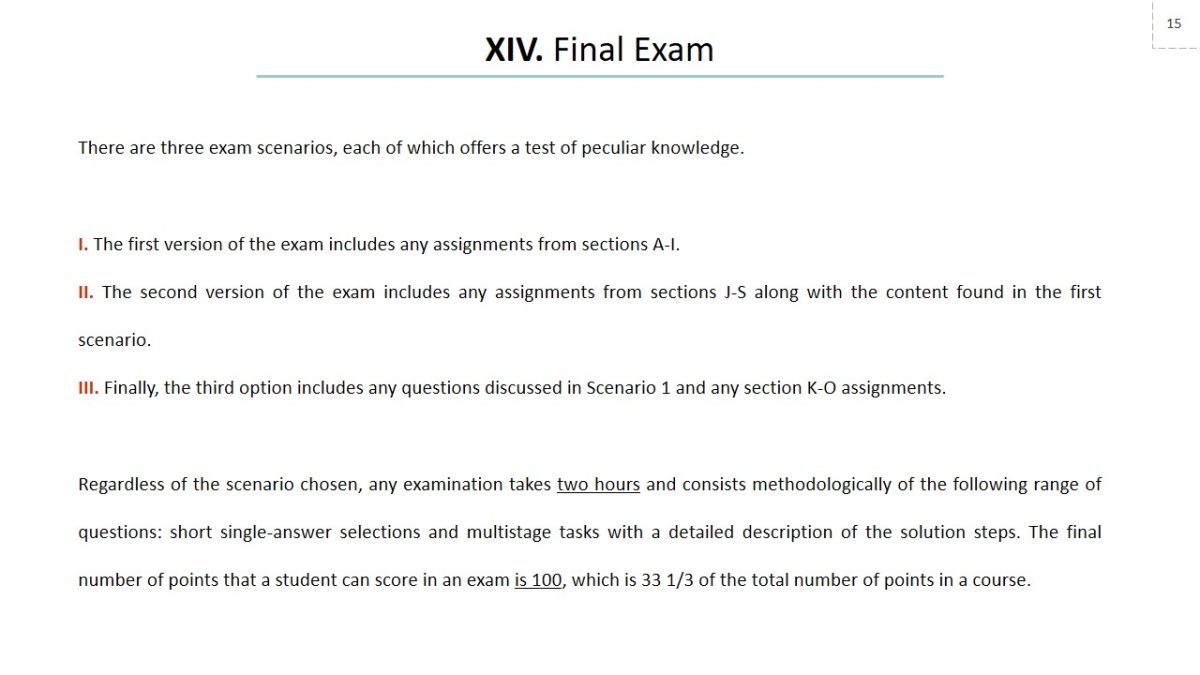
Final Exam

There are three exam scenarios, each of which offers a test of peculiar knowledge.

1. The first version of the exam includes any assignments from sections A-I.
2. The second version of the exam includes any assignments from sections J-S along with the content found in the first scenario.
3. Finally, the third option includes any questions discussed in Scenario 1 and any section K-O assignments.

Regardless of the scenario chosen, any examination takes two hours and consists methodologically of the following range of questions: short single-answer selections and multistage tasks with a detailed description of the solution steps. The final number of points that a student can score in an exam is 100, which is 33 1/3 of the total number of points in a course.

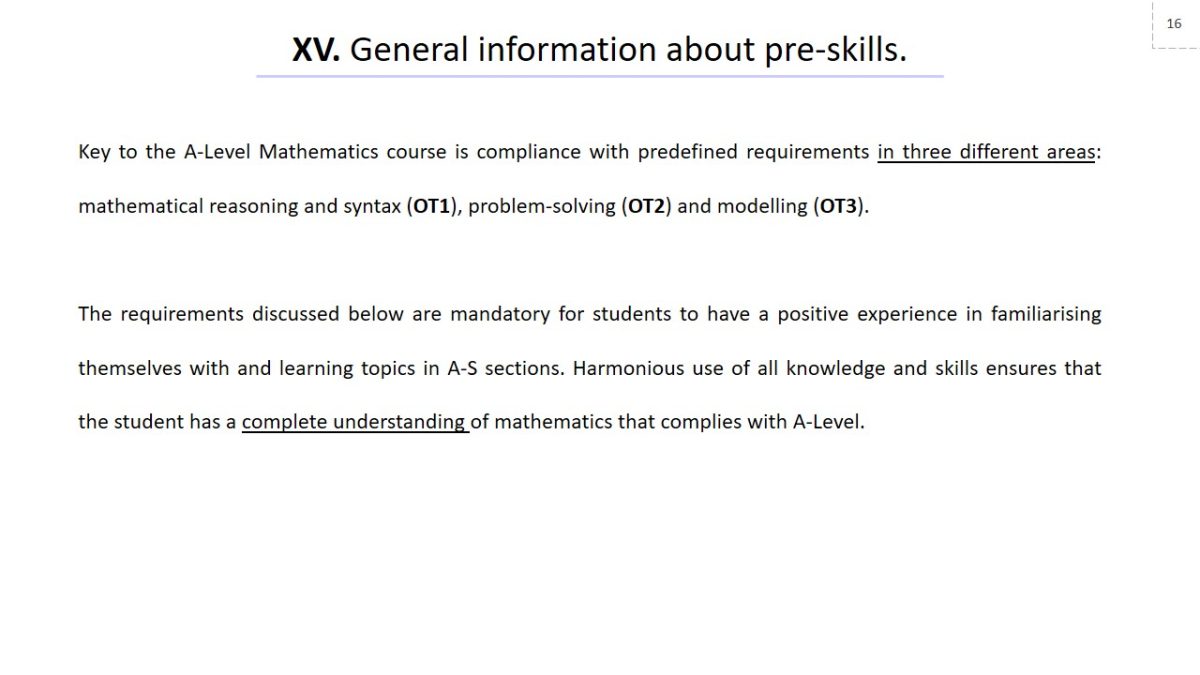
General information about pre-skills

Key to the A-Level Mathematics course is compliance with predefined requirements in three different areas: mathematical reasoning and syntax (OT1), problem-solving (OT2) and modelling (OT3).

The requirements discussed below are mandatory for students to have a positive experience in familiarising themselves with and learning topics in A-S sections. Harmonious use of all knowledge and skills ensures that the student has a complete understanding of mathematics that complies with A-Level.

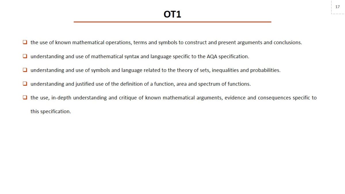
OT1

• The use of known mathematical operations, terms and symbols to construct and present arguments and conclusions.
• Understanding and use of mathematical syntax and language specific to the AQA specification.
• Understanding and use of symbols and language related to the theory of sets, inequalities and probabilities.
• Understanding and justified use of the definition of a function, area and spectrum of functions.
• The use, in-depth understanding and critique of known mathematical arguments, evidence and consequences specific to this specification.

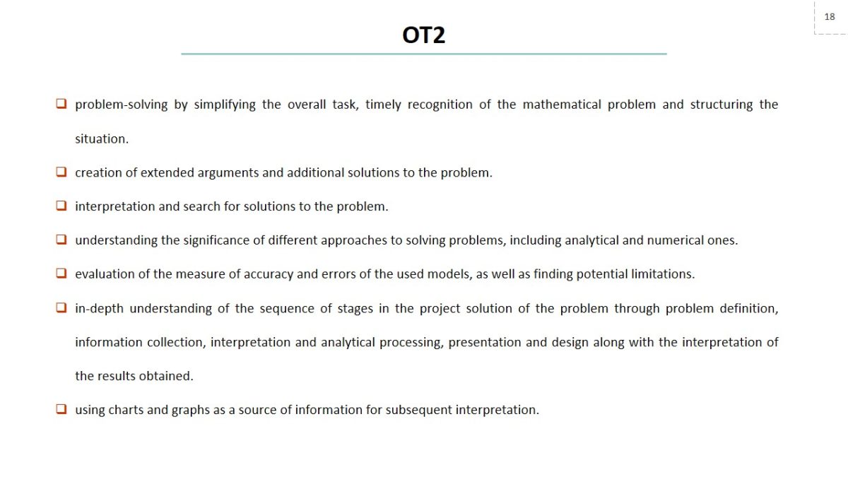
OT2

• Problem-solving by simplifying the overall task, timely recognition of the mathematical problem and structuring the situation.
• Creation of extended arguments and additional solutions to the problem.
• Interpretation and search for solutions to the problem.
• Understanding the significance of different approaches to solving problems, including analytical and numerical ones.
• Evaluation of the measure of accuracy and errors of the used models, as well as finding potential limitations.
• In-depth understanding of the sequence of stages in the project solution of the problem through problem definition, information collection, interpretation and analytical processing, presentation and design along with the interpretation of the results obtained.
• Using charts and graphs as a source of information for subsequent interpretation.

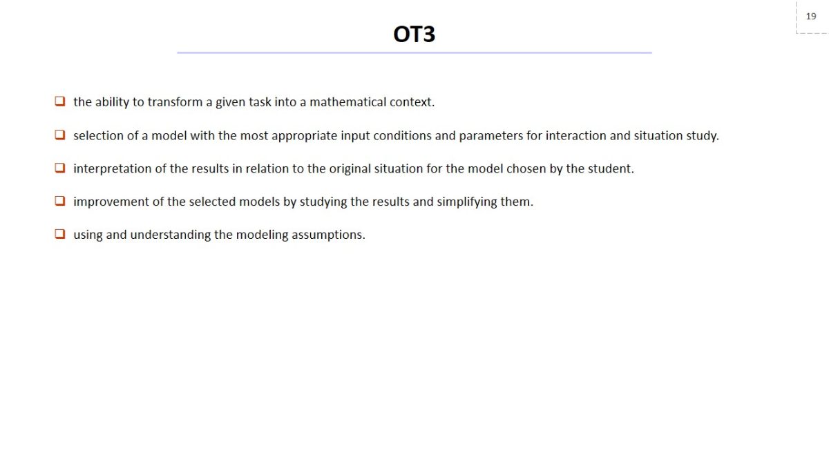
OT3

• The ability to transform a given task into a mathematical context.
• Selection of a model with the most appropriate input conditions and parameters for interaction and situation study.
• Interpretation of the results in relation to the original situation for the model chosen by the student.
• Improvement of the selected models by studying the results and simplifying them.
• Using and understanding the modeling assumptions.

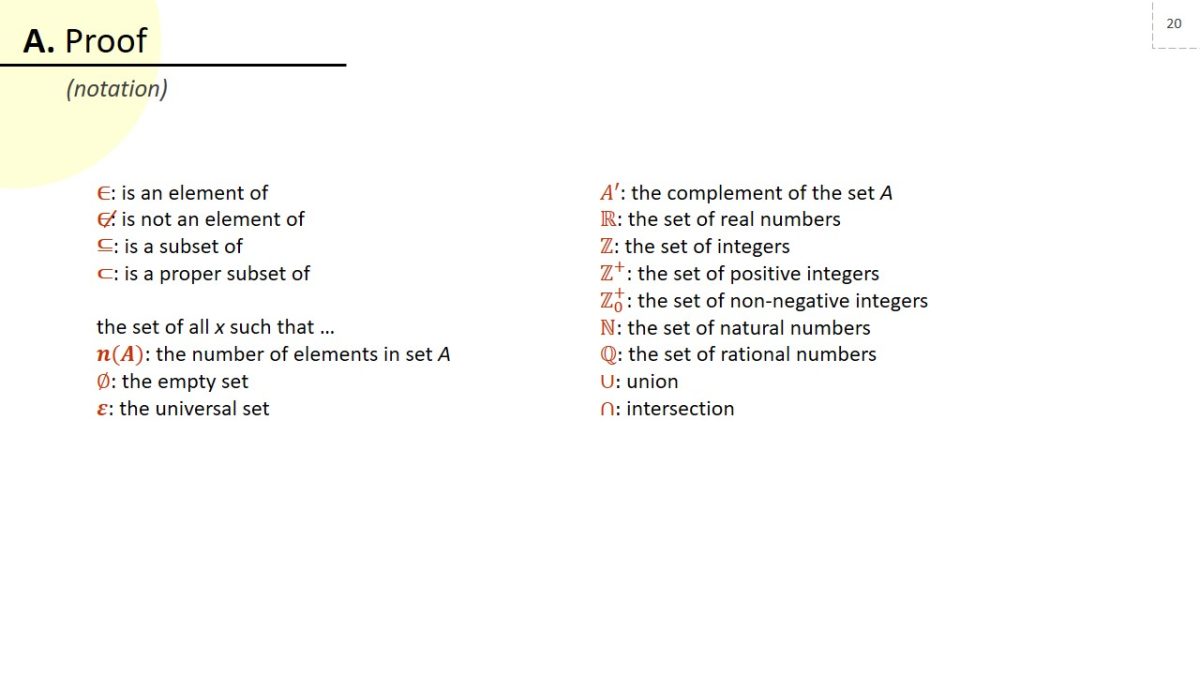
Proof

Notation

• ∈: is an element of;
• ∉: is not an element of;
• ⊆: is a subset of;
• ⊂: is a proper subset of the set of all x such that …
• n(A): the number of elements in set A;
• ∅: the empty set;
• ε: the universal set;
• A′: the complement of the set A;
• R: the set of real numbers;
• Z: the set of integers;
• Z^+: the set of positive integers;
• Z_0^+: the set of non-negative integers;
• N: the set of natural numbers;
• Q: the set of rational numbers;
• ∪: union;
• ∩: intersection.

Content objectives

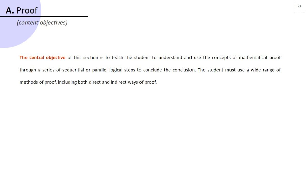
The central objective of this section is to teach the student to understand and use the concepts of mathematical proof through a series of sequential or parallel logical steps to conclude the conclusion. The student must use a wide range of methods of proof, including both direct and indirect ways of proof.

Example

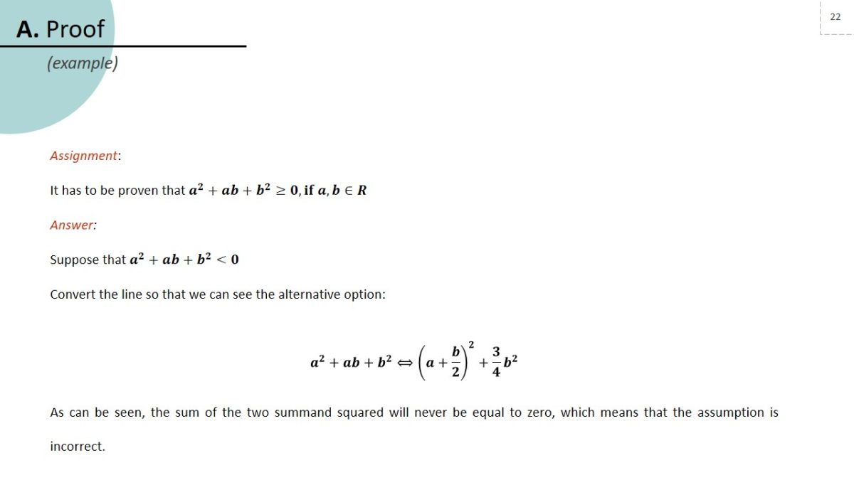
Assignment:

It has to be proven that a^2+ab+b^2≥0, if a,b∈R

Answer:

Suppose that a^2+ab+b^2<0

Convert the line so that we can see the alternative option:

a^2+ab+b^2⟺(a+b/2)^2+3/4 b^2

As can be seen, the sum of the two summand squared will never be equal to zero, which means that the assumption is incorrect.

Algebra and functions

Notation

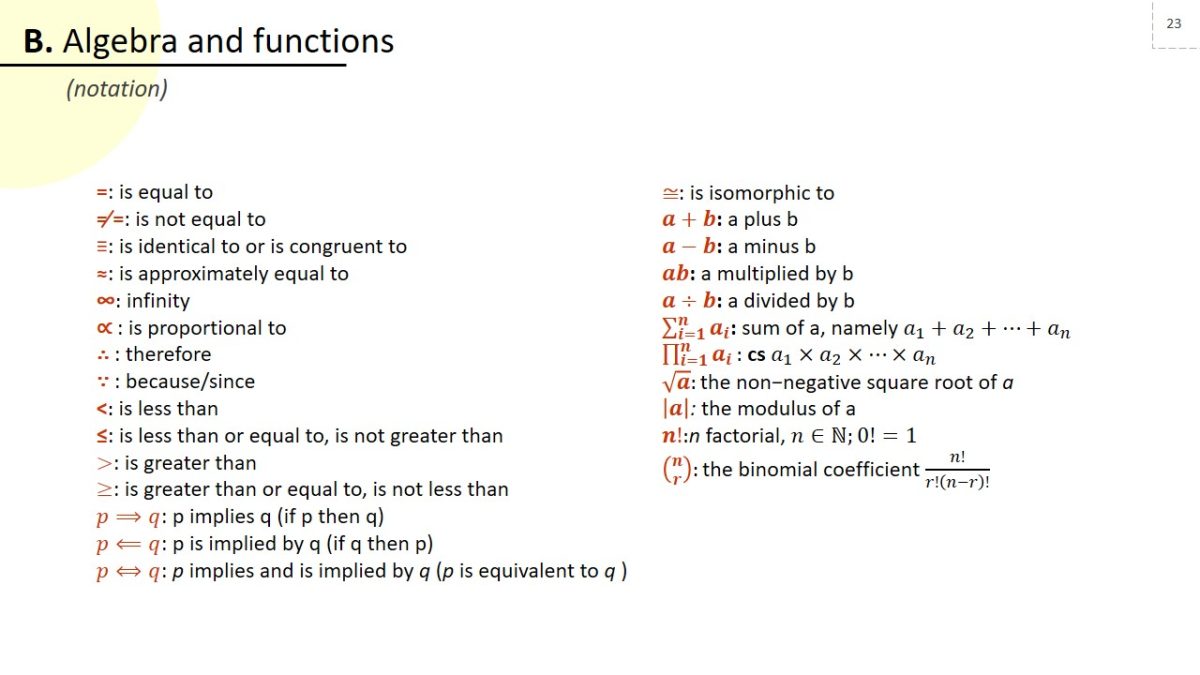
• =: is equal to
• ≠ =: is not equal to
• ≡: is identical to or is congruent to
• ≈: is approximately equal to
• “∞“: infinity
• ∝ : is proportional to
• ∴ : therefore
• ∵ : because/since
• “<“: is less than
• “≤“: is less than or equal to, is not greater than
• >: is greater than
• ≥: is greater than or equal to, is not less than
• p⟹q: p implies q (if p then q)
• p⟸q: p is implied by q (if q then p)
• p⟺q: p implies and is implied by q (p is equivalent to q )
• ≅: is isomorphic to
• a+b: a plus b
• a-b: a minus b
• ab: a multiplied by b
• a÷b: a divided by b
• ∑_(i=1)^n ai : sum of a, namely a_1+a_2+…+a_n
• ∏_(i=1)^n ai : cs a_1×a_2×…〖×a〗_n
• √a:“the non-negative square root of a”
• |a|: the modulus of a
• n!:n factorial, n∈N;0!=1
• (n¦r):“the binomial coefficient” n!/r!(n-r)!

Formulae and identities

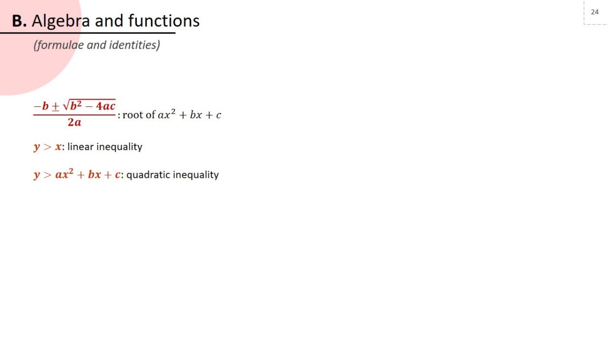
(-b±√(b^2-4ac))/2a : root of ax^2+bx+c

y>x: linear inequality.

y>ax^2+bx+c: quadratic inequality.

Content objectives

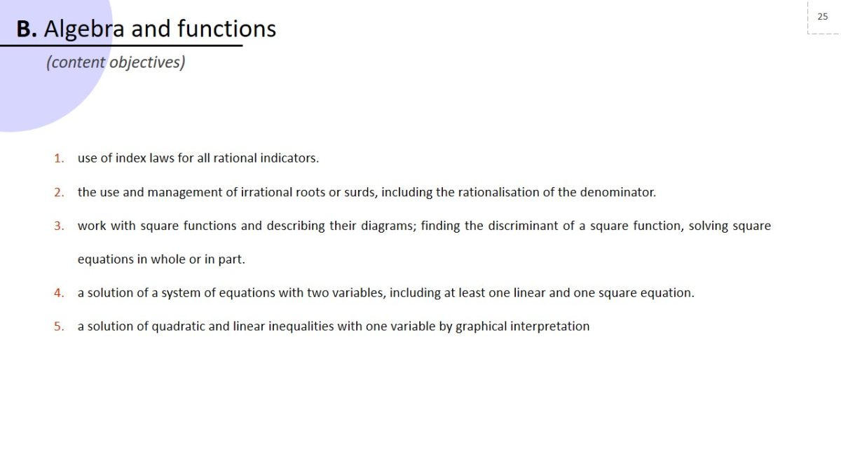
1. Use of index laws for all rational indicators.
2. The use and management of irrational roots or surds, including the rationalisation of the denominator.
3. Work with square functions and describing their diagrams; finding the discriminant of a square function, solving square equations in whole or in part.
4. A solution of a system of equations with two variables, including at least one linear and one square equation.
5. A solution of quadratic and linear inequalities with one variable by graphical interpretation.
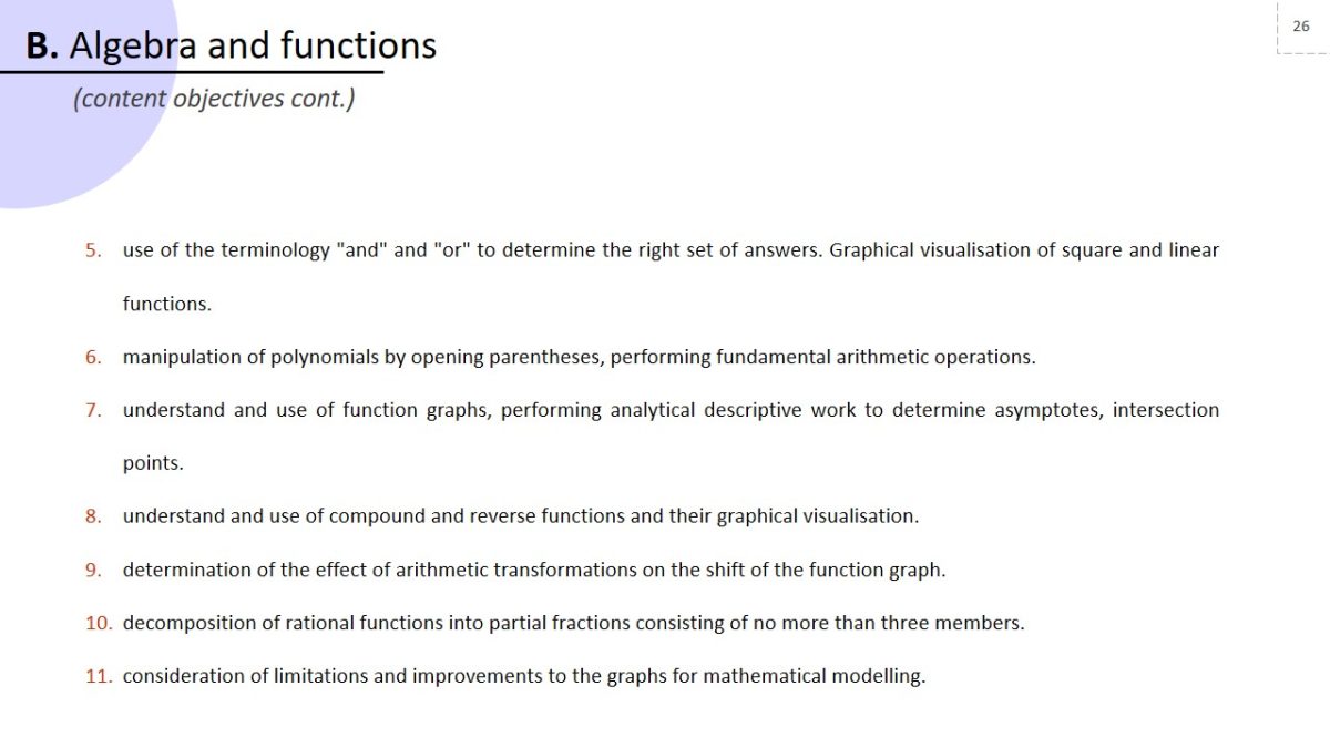
6. Use of the terminology “and” and “or” to determine the right set of answers. Graphical visualisation of square and linear functions.
7. Manipulation of polynomials by opening parentheses, performing fundamental arithmetic operations.
8. Understand and use of function graphs, performing analytical descriptive work to determine asymptotes, intersection points.
9. Understand and use of compound and reverse functions and their graphical visualisation.
10. Determination of the effect of arithmetic transformations on the shift of the function graph.
11. Decomposition of rational functions into partial fractions consisting of no more than three members.
12. Consideration of limitations and improvements to the graphs for mathematical modelling.

Example

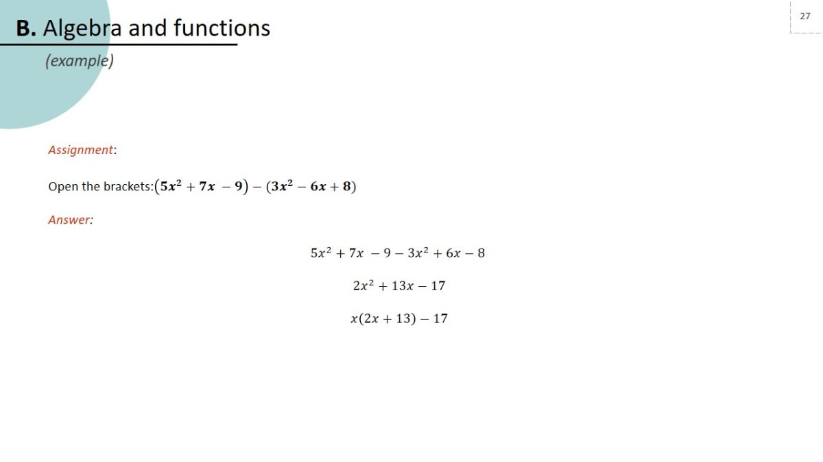
Assignment:

Open the brackets:(5x^2+7x -9)-(3x^2-6x+8).

Answer:

5x^2+7x -9-3x^2+6x-8;

2x^2+13x-17;

x(2x+13)-17.

Coordinate geometry in the (x, y) plane

Notation

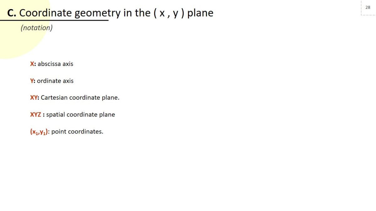
• X: abscissa axis.
• Y: ordinate axis.
• XY: Cartesian coordinate plane.
• XYZ: spatial coordinate plane
• (x1,y1): point coordinates.

Formulae and identities

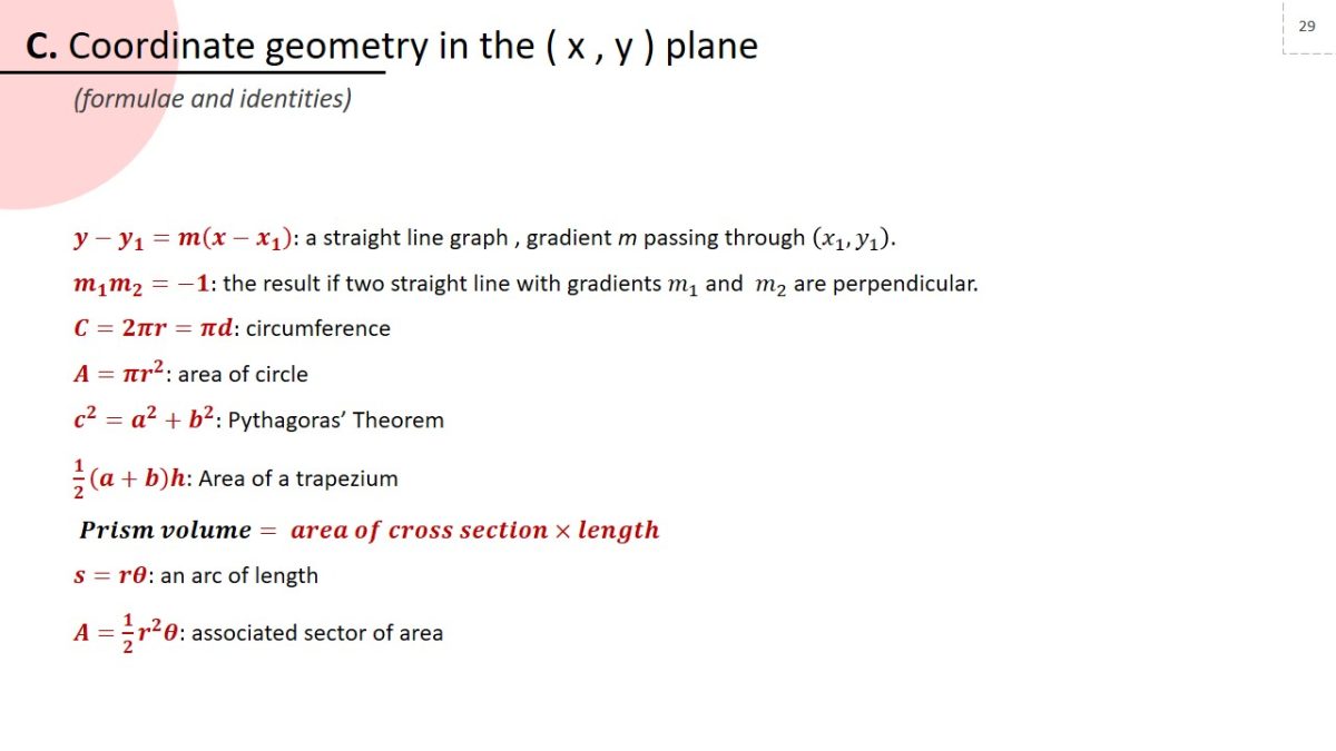
y-y_1=m(x-x_1 ): “a straight line graph , gradient m passing” through (x_1,y_1 ).

m_1 m_2=-1: the result if two straight line with gradients m_1 and m_2 are perpendicular.

C=2πr=πd: circumference.

A=πr^2: area of circle.

c^2=a^2+b^2: Pythagoras’ Theorem.

1/2 (a+b)h: Area of a trapezium.

Prism volume= area of cross section×length.

s=rθ: an arc of length.

A=1/2r^2 θ: associated sector of area.

Content objectives

1. Operate with straight-line equations, finding the gradient, determining the perpendicularity and parallelism of two straight lines.
2. Utilise circle geometry, including the properties of right angle, chord and perpendicularity of radius and tangent.
3. Understand and use of parametric equations, a transformation from Cartesian to parametric.
4. Use of the parametric system in modelling.

Example

Assignment:

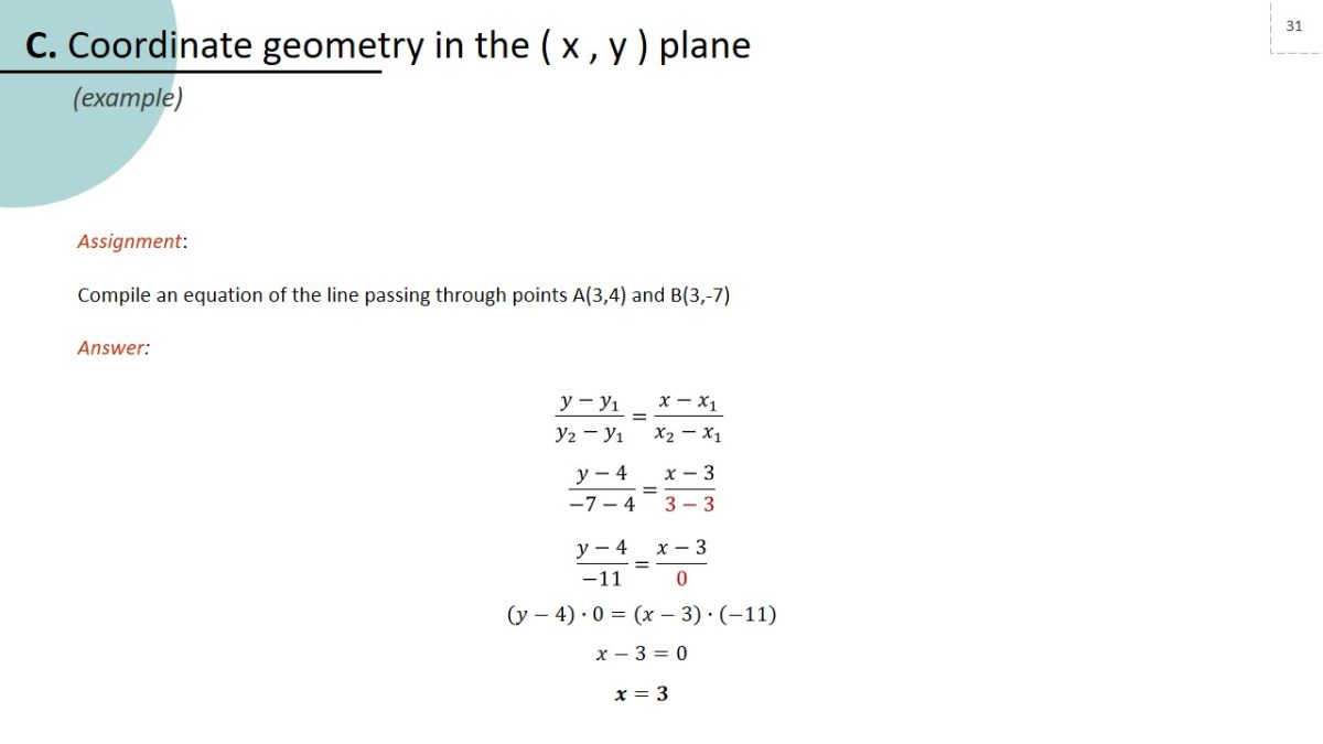
Compile an equation of the line passing through points A(3,4) and B(3,-7).

Answer:

(y-y_1)/(y_2-y_1 )=(x-x_1)/(x_2-x_1 )

(y-4)/(-7-4)=(x-3)/(3-3)

(y-4)/(-11)=(x-3)/0

(y-4)∙0=(x-3)∙(-11)

x-3=0

x=3

Sequences and series

Notation

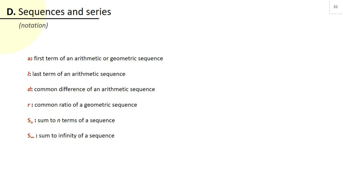
• a: first term of an arithmetic or geometric sequence.
• l: last term of an arithmetic sequence.
• d: common difference of an arithmetic sequence.
• r: common ratio of a geometric sequence.
• Sn : sum to n terms of a sequence.
• S∞ : sum to infinity of a sequence.

Formulae and identities

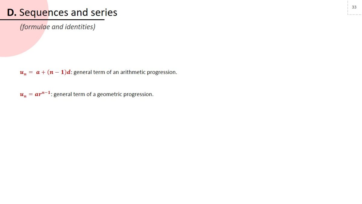
u_n= a+(n-1)d: general term of an arithmetic progression.

u_n=ar^(n-1): general term of a geometric progression.

Content objectives

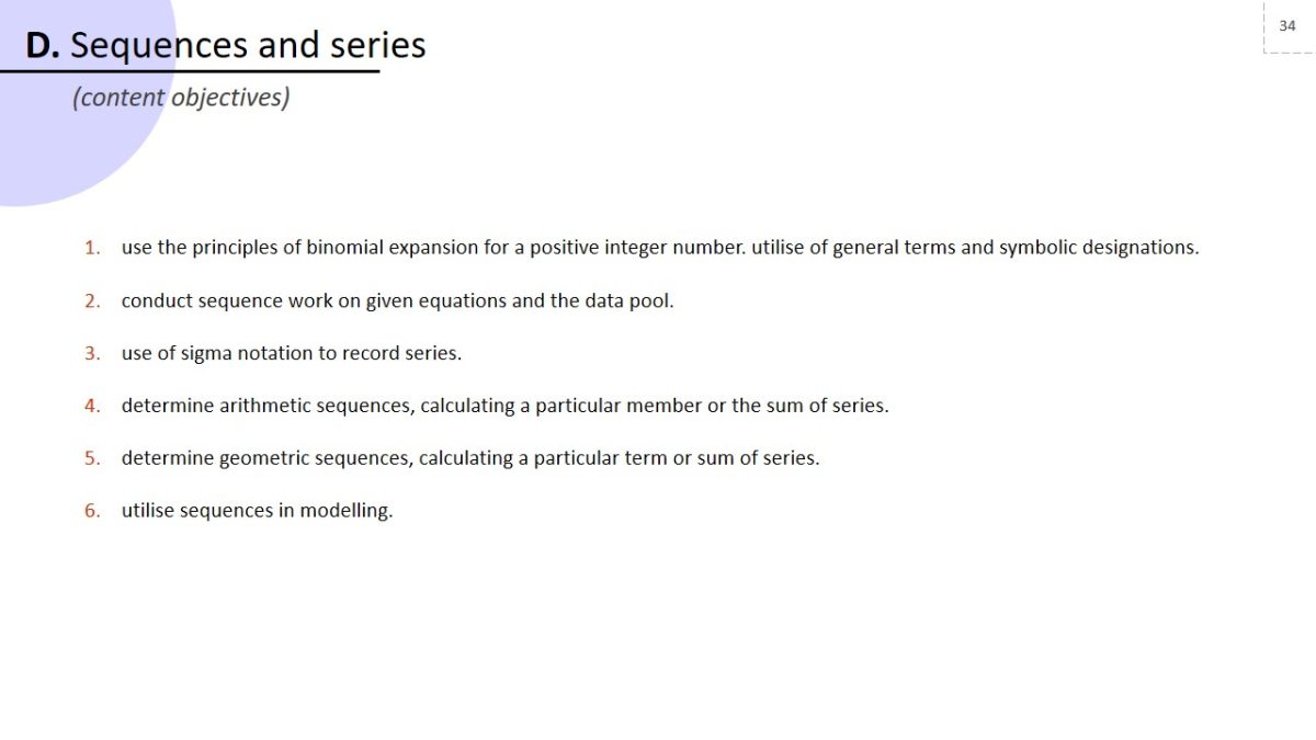
1. Use the principles of binomial expansion for a positive integer number. utilise of general terms and symbolic designations.
2. Conduct sequence work on given equations and the data pool.
3. Use of sigma notation to record series.
4. Determine arithmetic sequences, calculating a particular member or the sum of series.
5. Determine geometric sequences, calculating a particular term or sum of series.
6. Utilise sequences in modelling.

Example

Assignment:

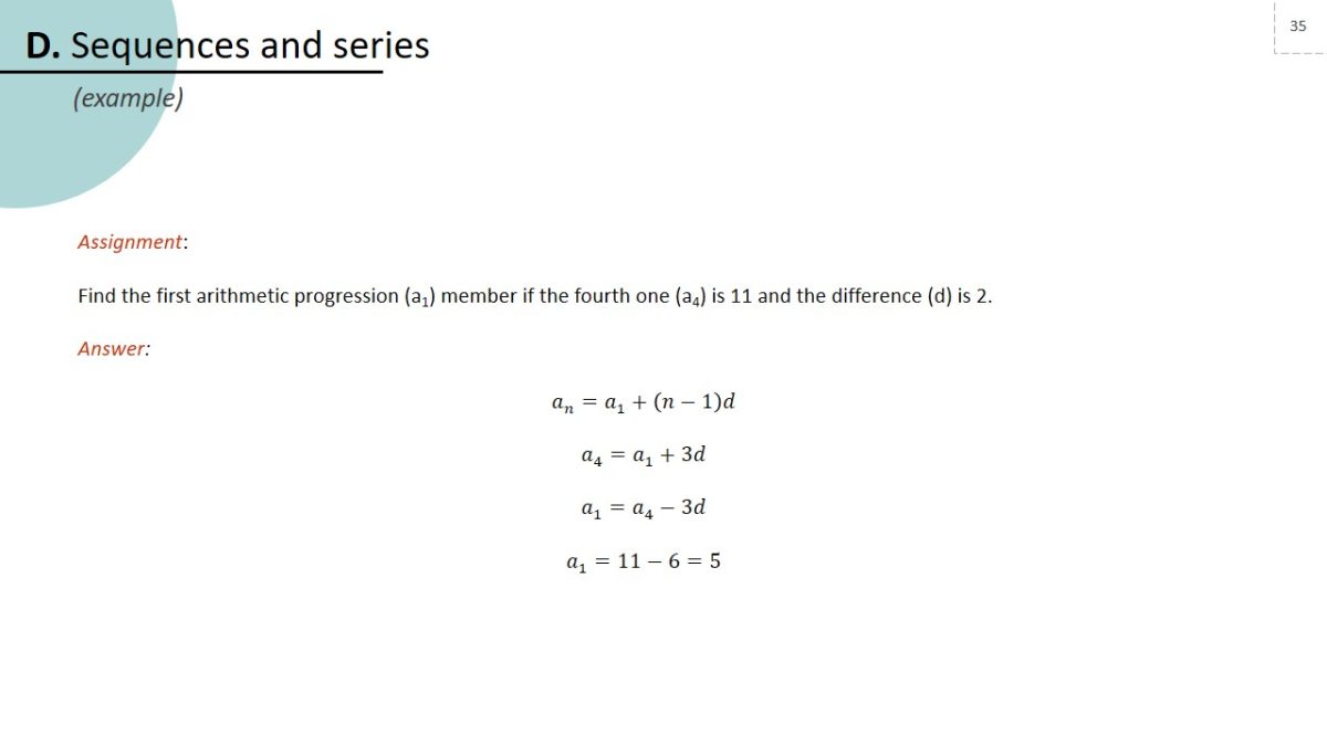
Find the first arithmetic progression (a1) member if the fourth one (a4) is 11 and the difference (d) is 2.

Answer:

an=a1+(n-1)d;

a4=a1+3d;

a1=a4-3d;

a1=11-6=5.

Trigonometry

Notation

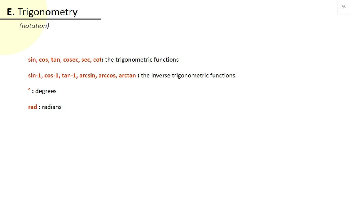
• sin, cos, tan, cosec, sec, cot: the trigonometric functions.
• sin-1, cos-1, tan-1, arcsin, arccos, arctan : the inverse trigonometric functions.
• ° : degrees.
• rad: radians.

Formulae and identities

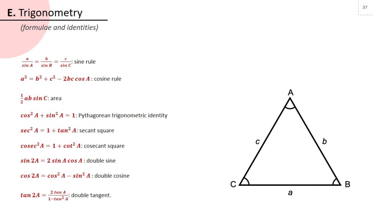
a/sin⁡A =b/sin⁡B =c/sin⁡C : sine rule.

a^2=b^2+c^2-2bc cos⁡A: cosine rule.

1/2 ab sin⁡C: area.

cos^2⁡A+sin^2⁡A=1: Pythagorean trigonometric identity.

sec^2⁡A=1+tan^2⁡A: secant square.

cosec^2 A=1+cot^2⁡A: cosecant square.

sin⁡2A=2 sin⁡A cos⁡A: double sine.

cos⁡2A=cos^2⁡A-sin^2⁡A: double cosine

tan⁡2A=(2 tan⁡A)/(1-tan^2⁡A ): double tangent.

Content objectives

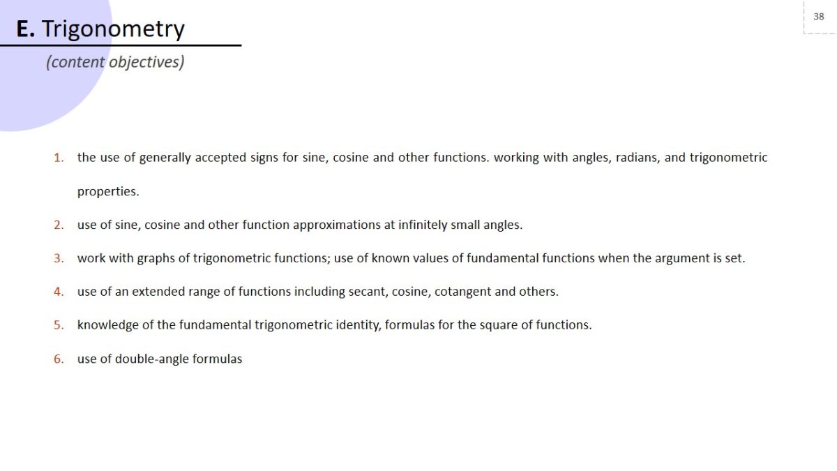
1. The use of generally accepted signs for sine, cosine and other functions. working with angles, radians, and trigonometric properties.
2. Use of sine, cosine and other function approximations at infinitely small angles.
3. Work with graphs of trigonometric functions; use of known values of fundamental functions when the argument is set.
4. Use of an extended range of functions including secant, cosine, cotangent and others.
5. Knowledge of the fundamental trigonometric identity, formulas for the square of functions.
6. Use of double-angle formulas
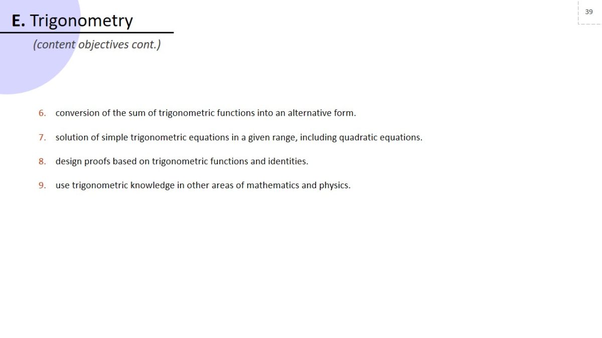
7. Conversion of the sum of trigonometric functions into an alternative form.
8. Solution of simple trigonometric equations in a given range, including quadratic equations.
9. Design proofs based on trigonometric functions and identities.
10. Use trigonometric knowledge in other areas of mathematics and physics.

Example

Assignment:

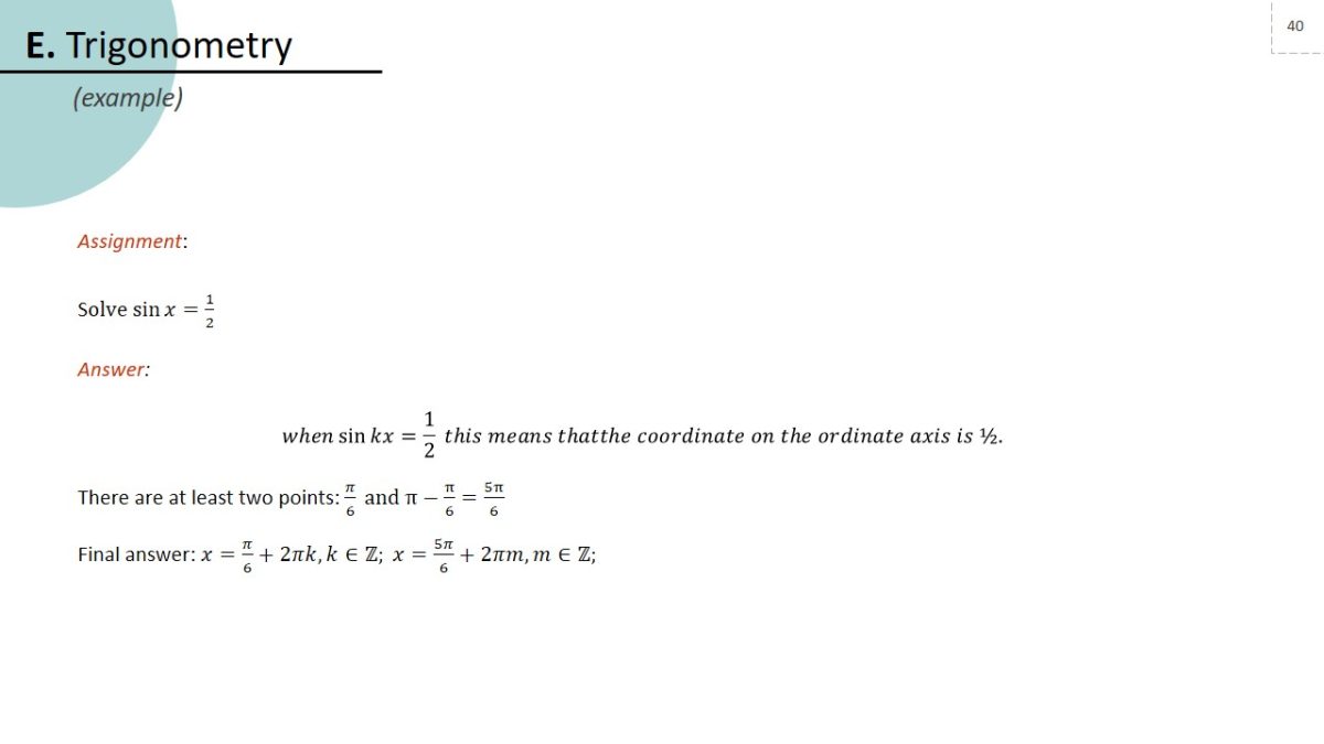
Solve sin⁡ x=1/2

Answer:

when sin⁡ kx=1/2 this means thatthe coordinate on the ordinate axis is ½.

There are at least two points: π/6 and π-π/6=5π/6.

Final answer: x=π/6+2πk, k∈Z; x=5π/6+2πm, m∈Z.

Exponentials and logarithms

Notation

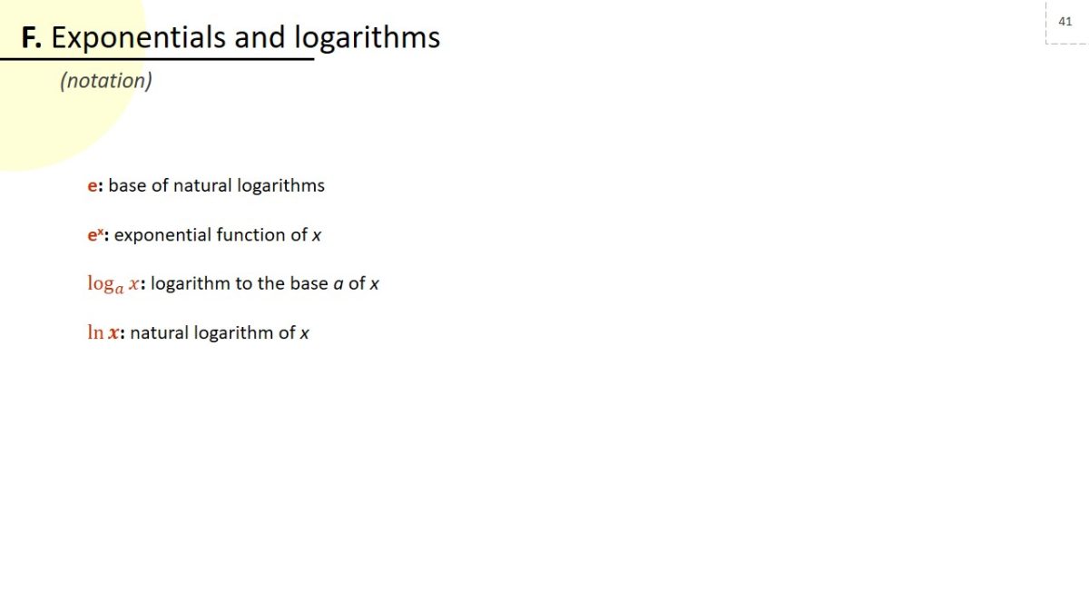
• e: base of natural logarithms.
• ex: exponential function of x .
• log a⁡ x: logarithm to the base a of x.
• ln⁡ x: natural logarithm of x.

Formulae and identities

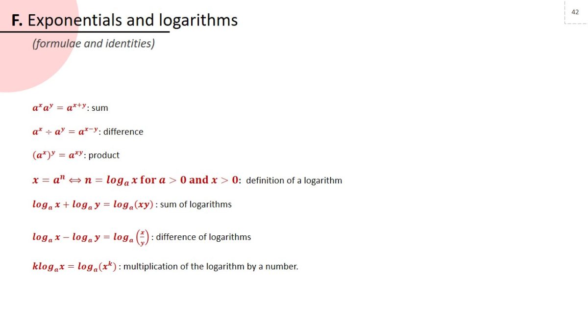
a^x a^y=a^(x+y): sum.

a^x÷a^y=a^(x-y): difference.

(a^x )^y=a^xy: product.

x=a^n⟺n=log_a⁡ x for a>0 and x>0:definition of a logarithm.

log_a⁡ x+log_a ⁡y=log_a⁡(xy) : sum of logarithms.

log_a⁡ x-log_a⁡ y=log_a⁡(x/y): difference of logarithms.

klog_a x=log_a⁡(x^k): multiplication of the logarithm by a number.

Content objectives

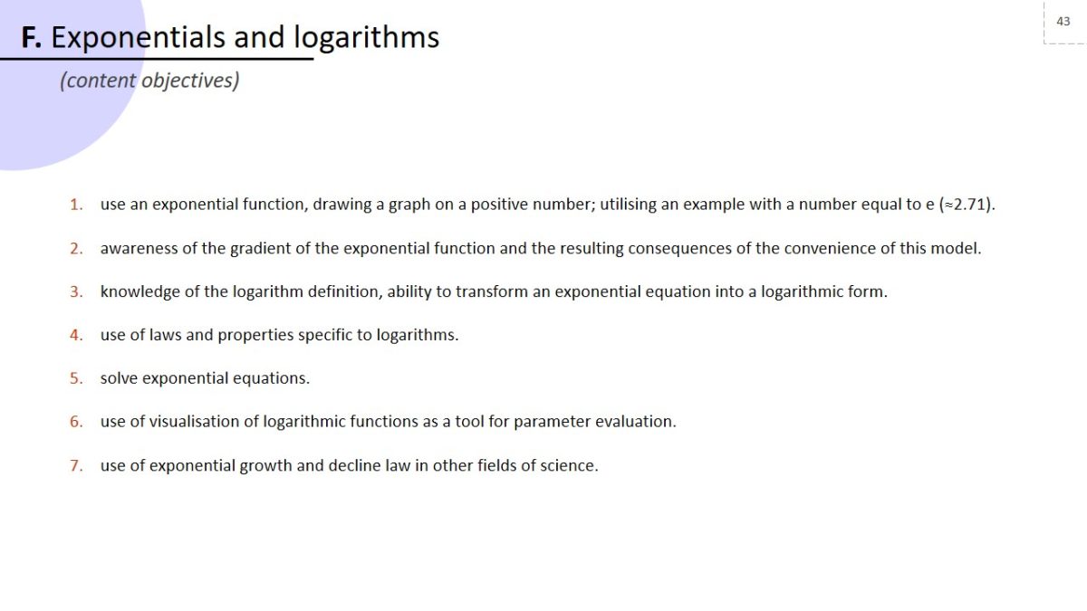
1. Use an exponential function, drawing a graph on a positive number; utilising an example with a number equal to e (≈2.71).
2. Awareness of the gradient of the exponential function and the resulting consequences of the convenience of this model.
3. Knowledge of the logarithm definition, ability to transform an exponential equation into a logarithmic form.
4. Use of laws and properties specific to logarithms.
5. Solve exponential equations.
6. Use of visualisation of logarithmic functions as a tool for parameter evaluation.
7. Use of exponential growth and decline law in other fields of science.

Example

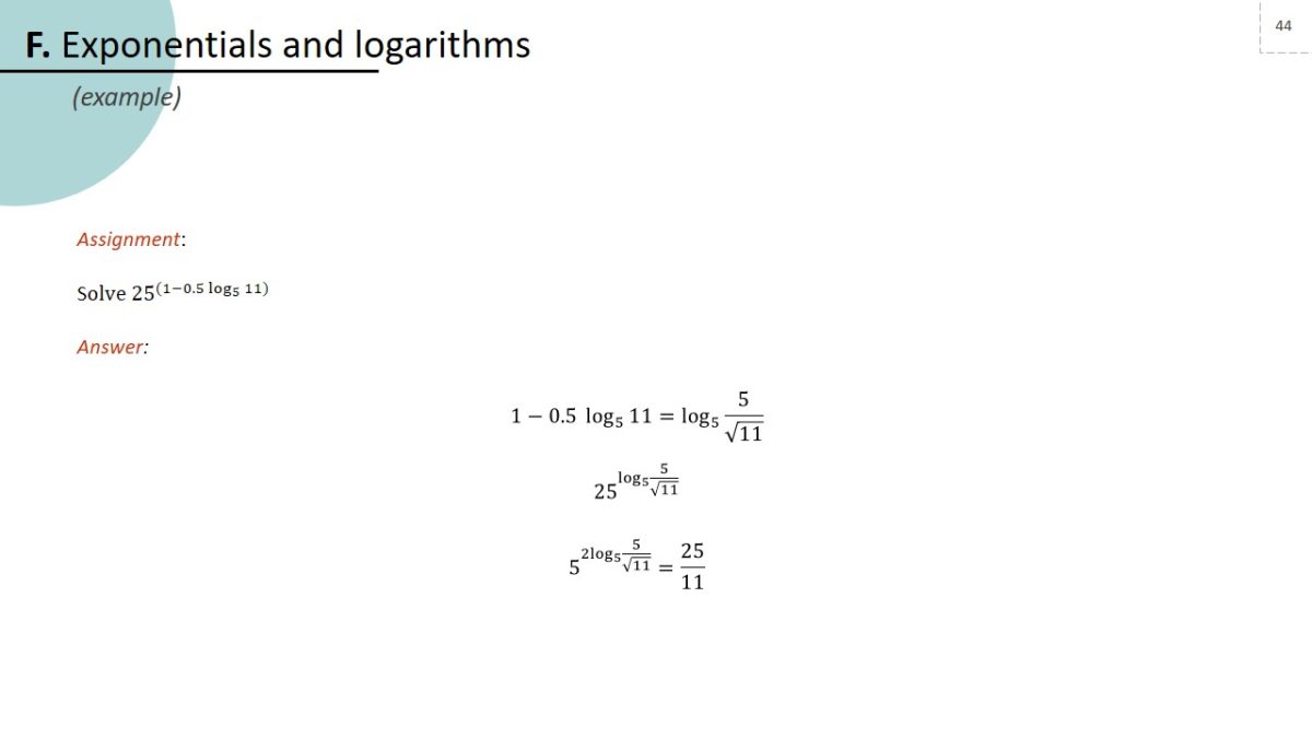
Assignment:

Solve 25^((1-0.5 log_5⁡ 11) )

Answer:

1-0.5 log_5⁡ 11=log_5⁡ 5/√11

25^log_5⁡ 5/√11

5^ 2 log_5⁡ 5/√11 =25/11

Differentiation

Notation

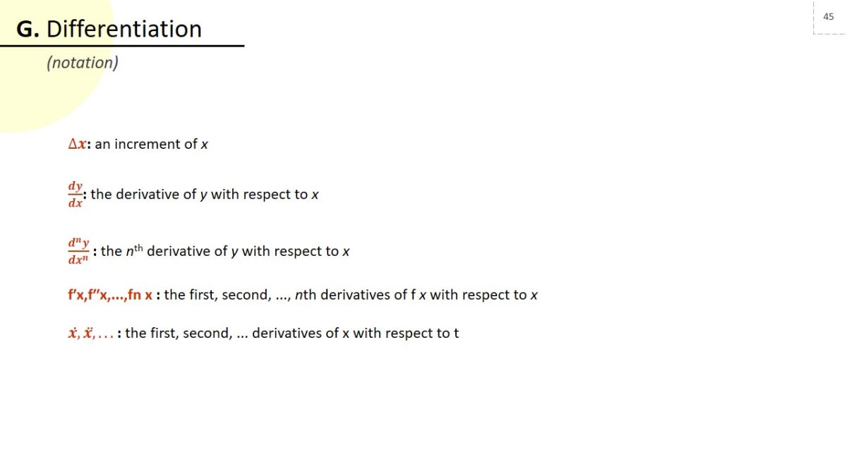
• ∆x“:“ an increment of x.
• dy/dx: the derivative of y with respect to x.
• (d^n y)/(dx^n ) : the nth derivative of y with respect to x.
• “f′x,f′′x,…,fn x “: the first, second, …, nth derivatives of f x with respect to x.
• ẋ,ẍ,… : the first, second, … derivatives of x with respect to t.

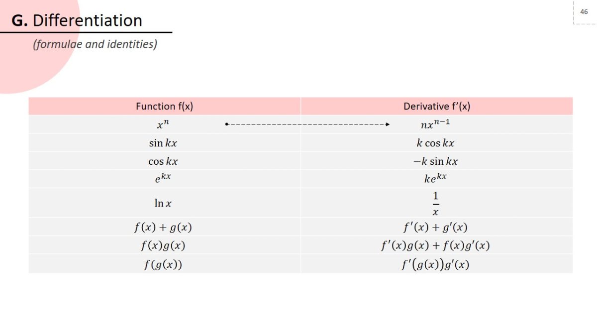
Formulae and identities

Content objectives

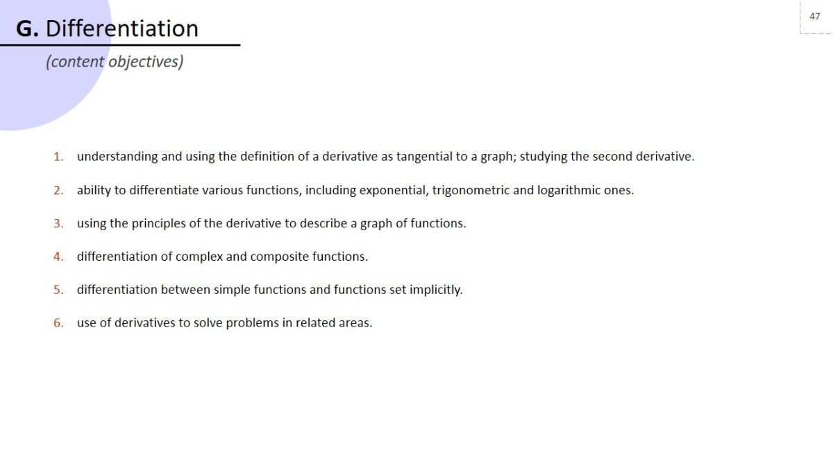
1. Understanding and using the definition of a derivative as tangential to a graph; studying the second derivative.
2. Ability to differentiate various functions, including exponential, trigonometric and logarithmic ones.
3. Using the principles of the derivative to describe a graph of functions.
4. Differentiation of complex and composite functions.
5. Differentiation between simple functions and functions set implicitly.
6. Use of derivatives to solve problems in related areas.

Example

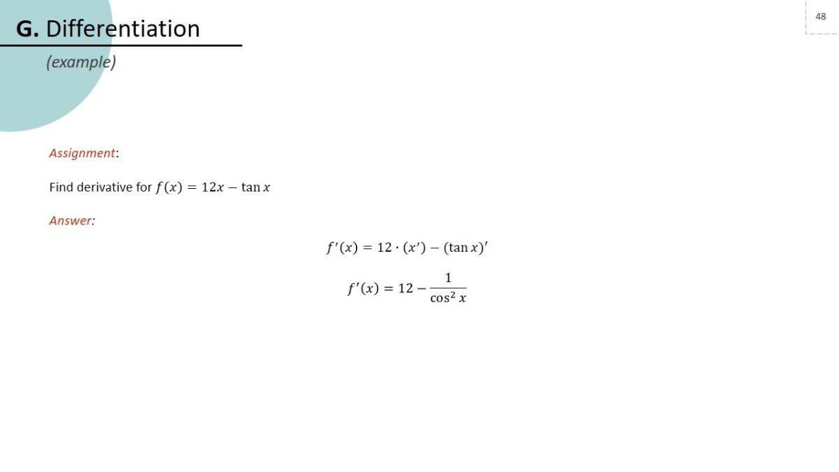
Assignment:

Find derivative for f(x)=12x-tan⁡x

Answer:

f^′ (x)=12∙(x^′ )-(tan x)′.

f^′ (x)=12-1/cos^2⁡x.

Integration

Notation

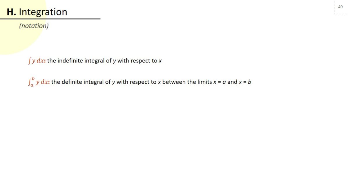
∫ y dx: the indefinite integral of y with respect to x.

∫_a^b y dx“:“ the definite integral of y with respect to x between the limits x = a and x = b.

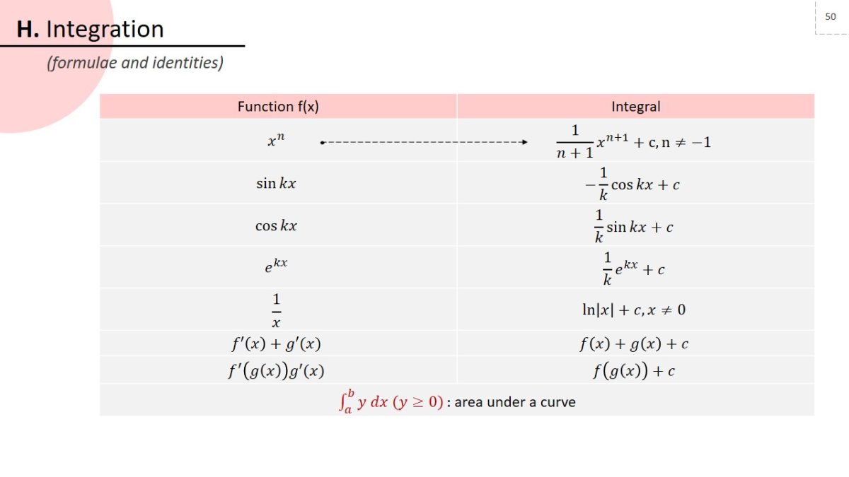
Formulae and identities

Content objectives

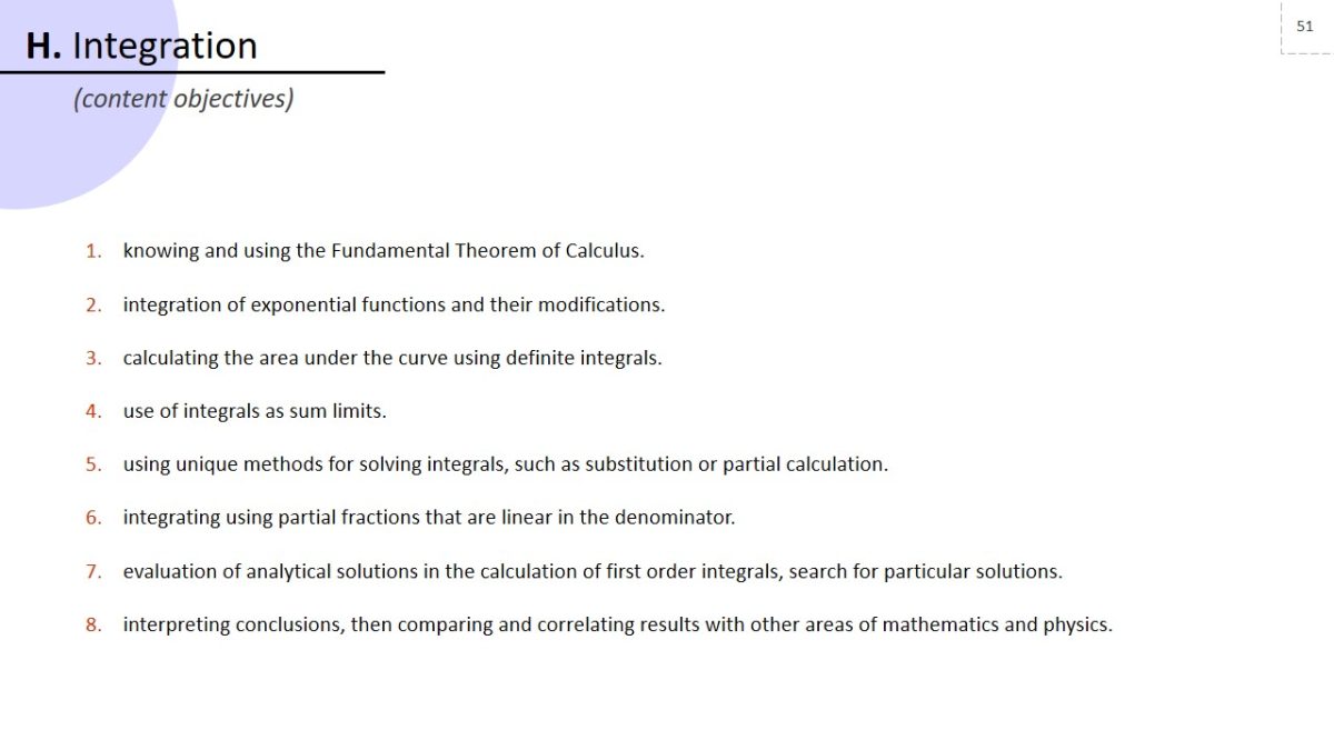
1. Knowing and using the Fundamental Theorem of Calculus.
2. Integration of exponential functions and their modifications.
3. Calculating the area under the curve using definite integrals.
4. Use of integrals as sum limits.
5. Using unique methods for solving integrals, such as substitution or partial calculation.
6. Integrating using partial fractions that are linear in the denominator.
7. Evaluation of analytical solutions in the calculation of first order integrals, search for particular solutions.
8. Interpreting conclusions, then comparing and correlating results with other areas of mathematics and physics.

Example

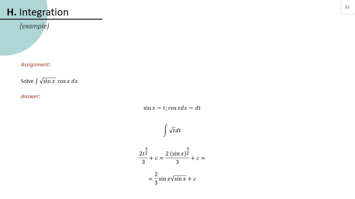
Assignment:

Solve ∫1√(sin ⁡x ) cos⁡ x dx

Answer:

sin⁡ x=t; cos⁡ x dx=dt

∫√t dt

(2t^(3/2))/3+c=(2 (sin x)^(3/2))/3+c = 2/3 sin⁡ x√(sin⁡x )+c.

Numerical methods

Content objectives

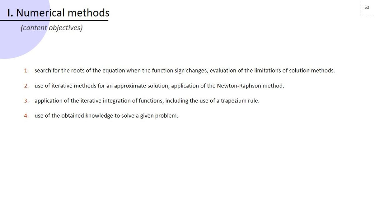
1. Search for the roots of the equation when the function sign changes; evaluation of the limitations of solution methods.
2. Use of iterative methods for an approximate solution, application of the Newton-Raphson method.
3. Application of the iterative integration of functions, including the use of a trapezium rule.
4. Use of the obtained knowledge to solve a given problem.

Example

Assignment:

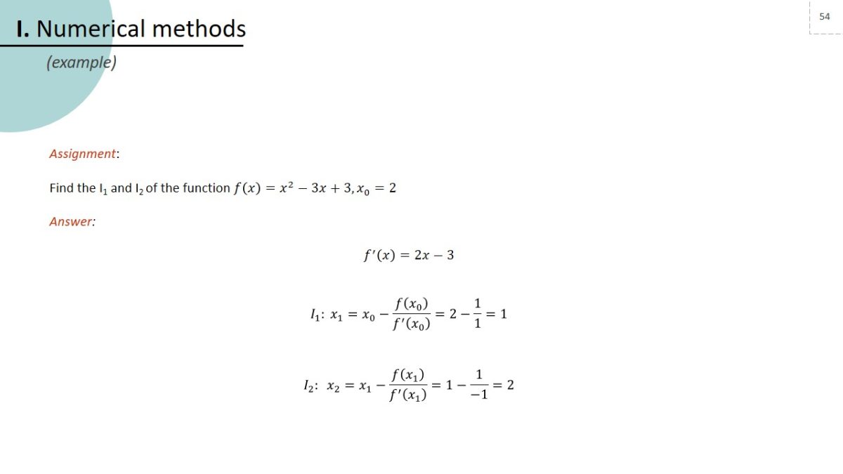
Find the I1 and I2 of the function f(x)=x^2-3x+3, x_0=2.

Answer:

f^′ (x)=2x-3

I_1: x_1=x_0-f(x_0 )/(f^′ (x_0 ) )=2-1/1=1.

I_2: x_2=x_1-f(x_1 )/(f^′ (x_1 ) )=1-1/(-1)=2.

Vectors

Notation

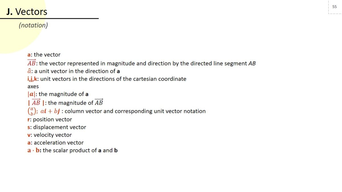
• a: the vector.
• (AB)→: the vector represented in magnitude and direction by the directed line segment AB.
• a ̂: a unit vector in the direction of a.
• i,j,k: unit vectors in the directions of the cartesian coordinate axes.
• |a|: the magnitude of a.
• | (AB)→ |: the magnitude of (AB).
• (a¦b); ai+bj : column vector and corresponding unit vector notation.
• r: position vector.
• s: displacement vector.
• v: velocity vector.
• a: acceleration vector.
• a∙b: the scalar product of a and b.

Formulae and identities

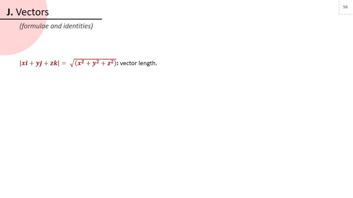
|xi+yj+zk|= √((x^2+y^2+z^2 ) ): vector length.

Content objectives

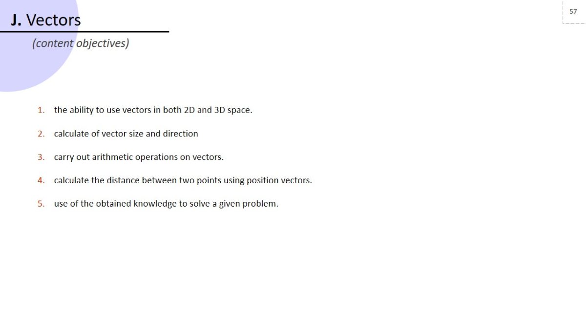
1. The ability to use vectors in both 2D and 3D space.
2. Calculate of vector size and direction
3. Carry out arithmetic operations on vectors.
4. Calculate the distance between two points using position vectors.
5. Use of the obtained knowledge to solve a given problem.

Example

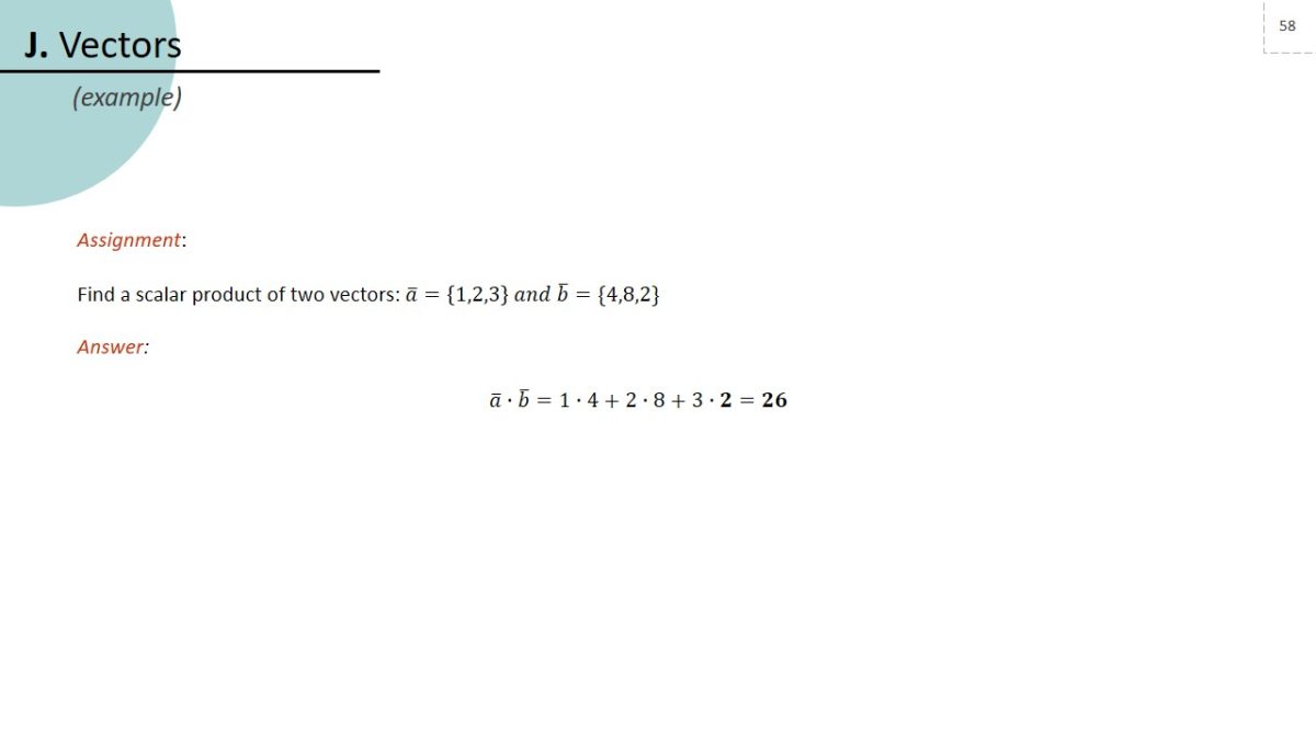
Assignment:

Find a scalar product of two vectors: a ̅= and b ̅=

Answer:

a ̅∙b ̅= 1∙4+2∙8+3∙2 = 26.

Statistical sampling

Notation

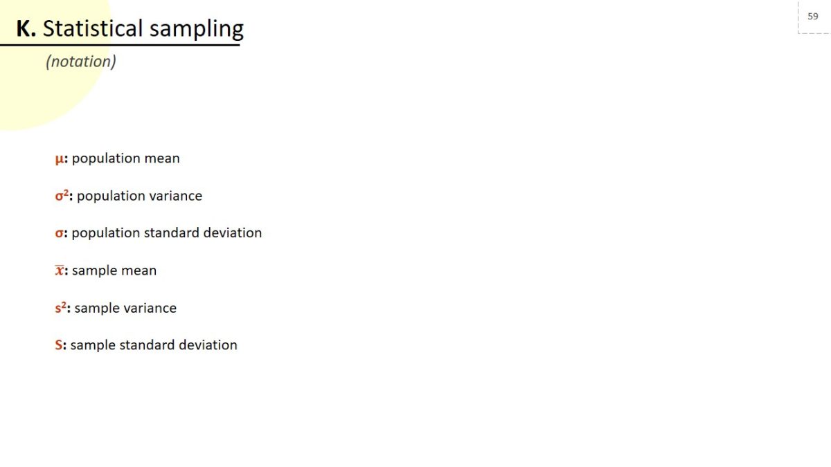
• µ: population mean.
• σ2: population variance.
• σ: population standard deviation.
• x ̅ : sample mean.
• s2: sample variance.
• S: sample standard deviation.

Formulae and identities

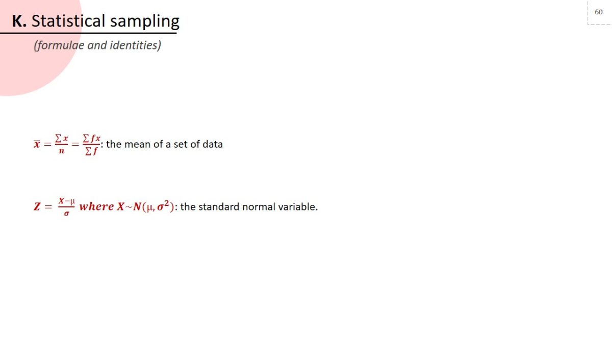
x ̅=(∑x)/n=(∑fx)/(∑f): the mean of a set of data.

Z= (X-µ)/σ where X~N(µ,σ^2): the standard normal variable.

Content objectives

Utilize the terms “sample” and “population” with confidence, conduct simple statistical analysis, have an understanding of sampling methods and critique them.

Example

Assignment:

There are 36 cards in the deck, nine of each suit. How many options are there to make a set of six cards consisting of two kings, one queen and three nines?

Answer:

• C_4^2 (kings)=6.
• C_4^3 (nines)=3.
• C_4^1 (queen)=4.
• N_cards=6×3×4=72.

Data presentation and interpretation

Content objectives

1. Interpret single-variable charts, including frequency distribution histograms.
2. Use scatter plots and linear regression analysis, perform correlation.
3. Interpret measures of central trend and variation, expanding them to standard deviation.
4. Consider potential sample limitations, critique existing methods, cleanse data from noise and calculate errors.

Example

Assignment:

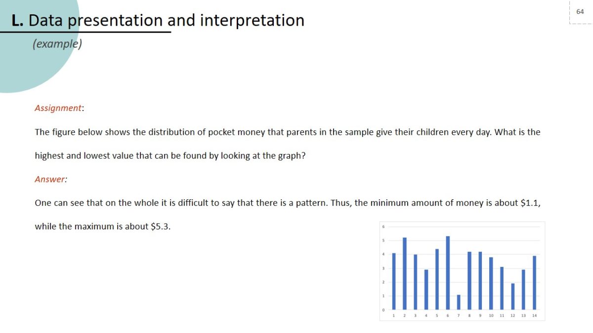
The figure below shows the distribution of pocket money that parents in the sample give their children every day. What is the highest and lowest value that can be found by looking at the graph?

Answer:

One can see that on the whole it is difficult to say that there is a pattern. Thus, the minimum amount of money is about $1.1, while the maximum is about $5.3.

Probability

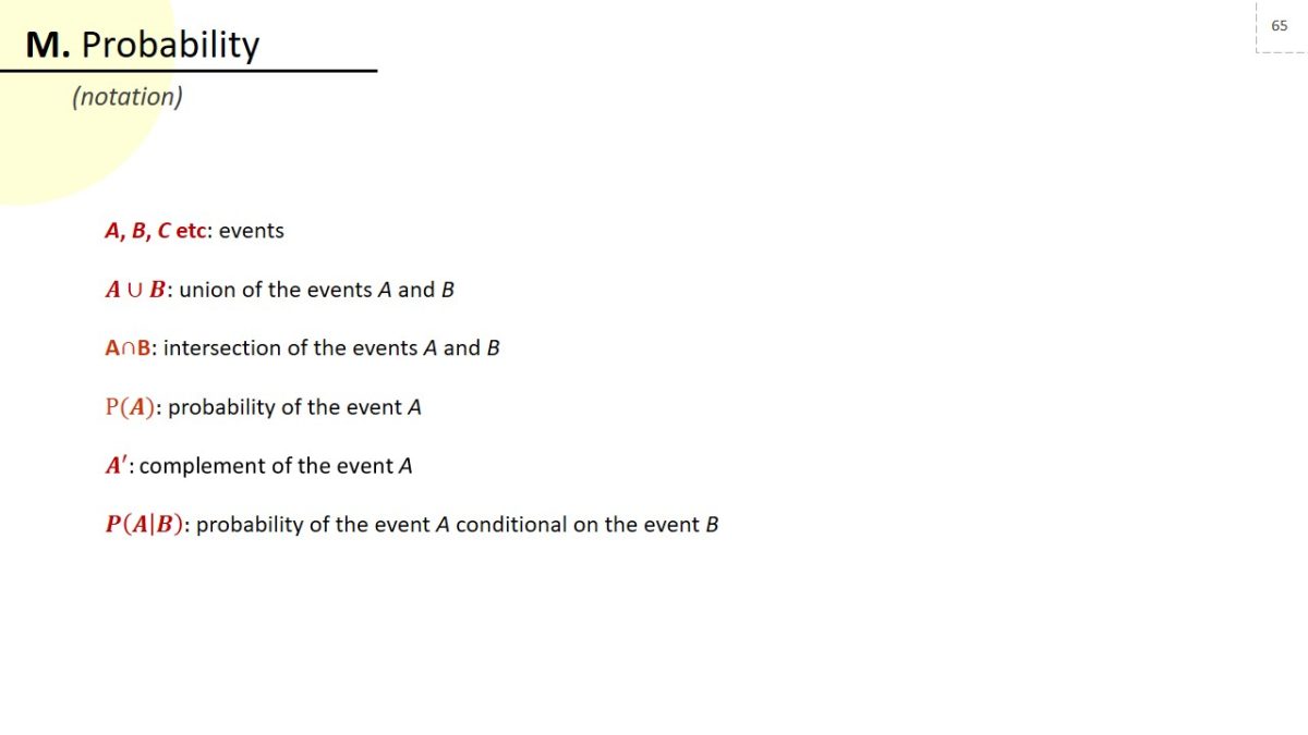
Notation

• A, B, C etc: events.
• A∪B: union of the events A and B.
• A∩B: intersection of the events A and B.
• P(A): probability of the event A.
• A^′:“complement of the event A”.
  
• P(A│B): probability of the event A conditional on the event B.

Formulae and identities

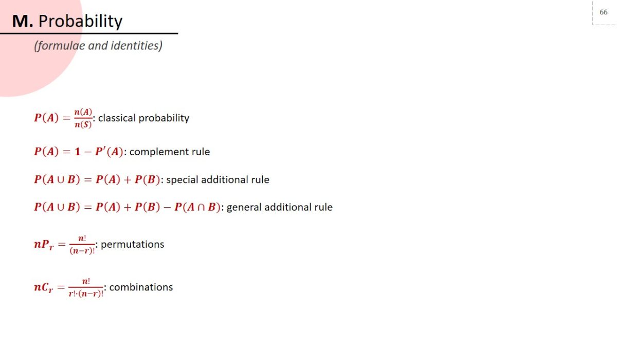
• P(A)=n(A)/n(S) : classical probability.
• P(A)=1-P^′ (A): complement rule.
• P(A∪B)=P(A)+P(B): special additional rule.
• P(A∪B)=P(A)+P(B)-P(A∩B): general additional rule.
• nP_r=n!/(n-r)!: permutations.
• nC_r=n!/(r!∙(n-r)!): combinations.

Content objectives

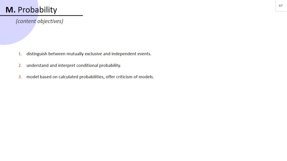
1. Distinguish between mutually exclusive and independent events.
2. Understand and interpret conditional probability.
3. Model based on calculated probabilities, offer criticism of models.

Example

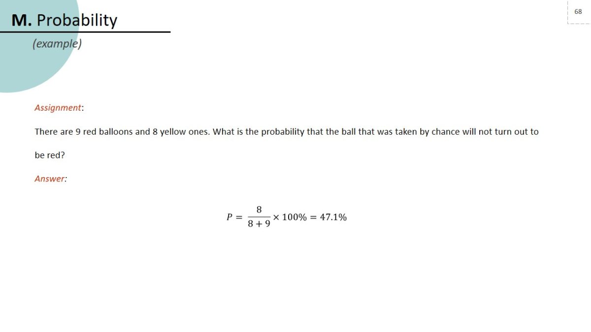
Assignment:

There are 9 red balloons and 8 yellow ones. What is the probability that the ball that was taken by chance will not turn out to be red?

Answer:

P= 8/(8+9)×100%=47.1%

Statistical distributions

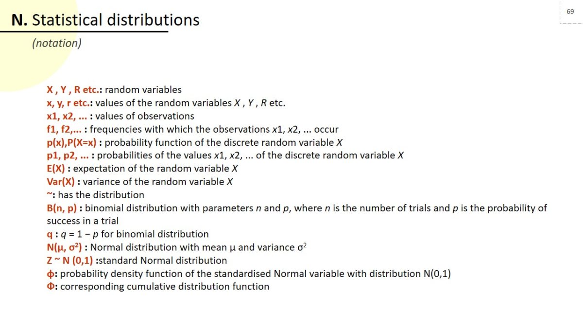
Notation

• X , Y , R etc.: random variables.
• x, y, r etc.: values of the random variables X , Y , R etc.
• x1, x2, … : values of observations.
• f1, f2,… : frequencies with which the observations x1, x2, … occur.
• p(x),P(X=x) : probability function of the discrete random variable X.
• p1, p2, … : probabilities of the values x1, x2, … of the discrete random variable X.
• E(X) : expectation of the random variable X.
• Var(X) : variance of the random variable X.
• ~: has the distribution.
• B(n, p) : binomial distribution with parameters n and p, where n is the number of trials and p is the probability of success in a trial.
• q : q = 1 − p for binomial distribution.
• N(µ, σ2) : Normal distribution with mean µ and variance σ2.
• Z ~ N (0,1) :standard Normal distribution.
• φ: probability density function of the standardised Normal variable with distribution N(0,1).
• Ф: corresponding cumulative distribution function.

Content objectives

1. Understand simple probability distributions, including the calculation of the mean and dispersion of discrete random variables.
2. Familiarise with the normal distribution, use it as a model.
3. Selecting specific distribution models, depending on the context of the task at hand.

Example

Assignment:

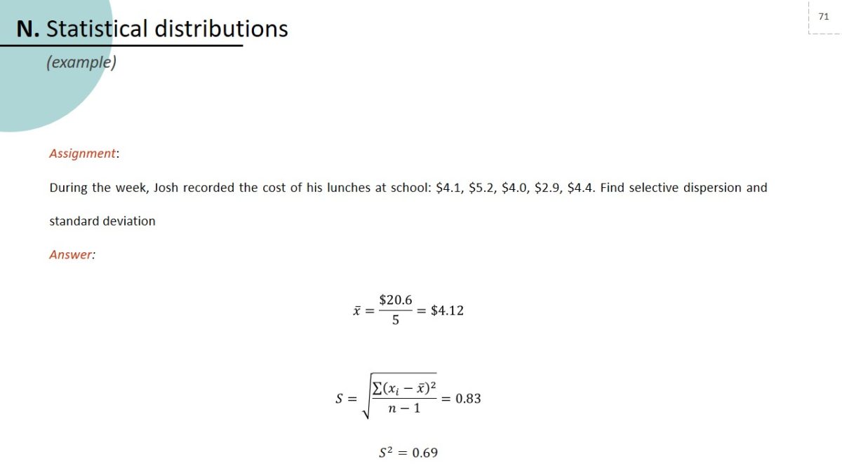
During the week, Josh recorded the cost of his lunches at school: $4.1, $5.2, $4.0, $2.9, $4.4. Find selective dispersion and standard deviation.

Answer:

x ̅=$20.6/5=$4.12.

S=√((∑(x_i-x ̅ )^2 )/(n-1))=0.83.

S^2=0.69.

Statistical hypothesis testing

Notation

• H0: null hypothesis.
• H1: alternative hypothesis.
• r: product moment correlation coefficient for a sample.
• ρ: product moment correlation coefficient for a population.

Content objectives

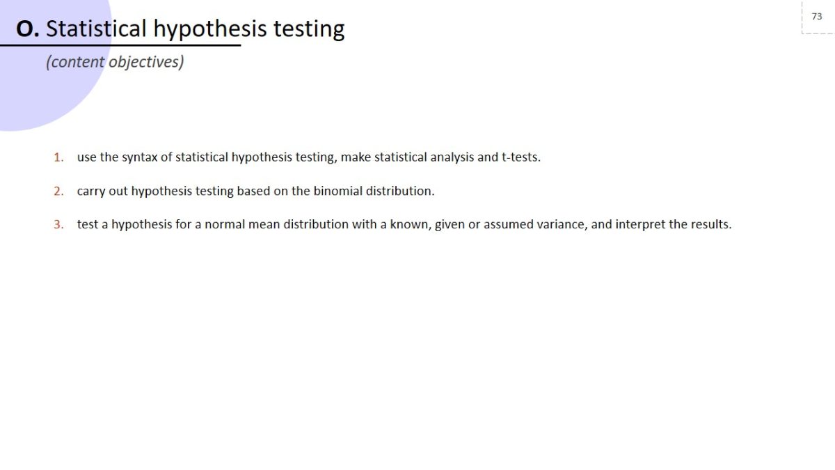
1. Use the syntax of statistical hypothesis testing, make statistical analysis and t-tests.
2. Carry out hypothesis testing based on the binomial distribution.
3. Test a hypothesis for a normal mean distribution with a known, given or assumed variance, and interpret the results.

Example

Assignment:

The seller claims that the average weight of a package of Coca-Cola tea is 300 g. A sample was taken from the batch and weighed. The weight of each can was counted and averaged. Does this not contradict the seller’s statement? There is a 99% confidence probability. The weight of the Coca-Cola is distributed normally.

Answer:

H_0:a=300;H_1:a≠300

x ̅=299.63

S= √(1/(n-1) ∑(x_i-x ̅ )^2 )=2.81

T= ((x ̅-a))/S √n=((299.63-300))/2.81 √9=-0.40

-0.40<3.3554 (from table)

H0 is accepted.

Quantities and units in mechanics

Notation

• kg: kilogram.
• m: metre.
• km: kilometre.
• m/s: metre(s) per second.
• “m/s” 2: metre(s) per second per second.

Formulae and identities

• F_net=ma: net force.
• F_f=µF_N: friction force.
• a_c=v^2/r: centripetal acceeration.
• J=F∆t=m∆v“:” impulse.
• W=F∆x: mechanical work.

Content objectives

Have an understanding of fundamental physical quantities and units of measurement in SI; use derivatives of these quantities.

Example

Assignment:

There is a laptop massed 1.1 kg on the table. Determine the weight of the device.

Answer:

P=mg

P = 1.1 ∙ 9.81 = 10.79 N.

Kinematics

Notation

• t: time.
• s: displacement.
• u: initial velocity.
• v: velocity or final velocity.
• a: acceleration.
• g: acceleration due to gravity.
• µ: coefficient of friction.

Formulae and identities

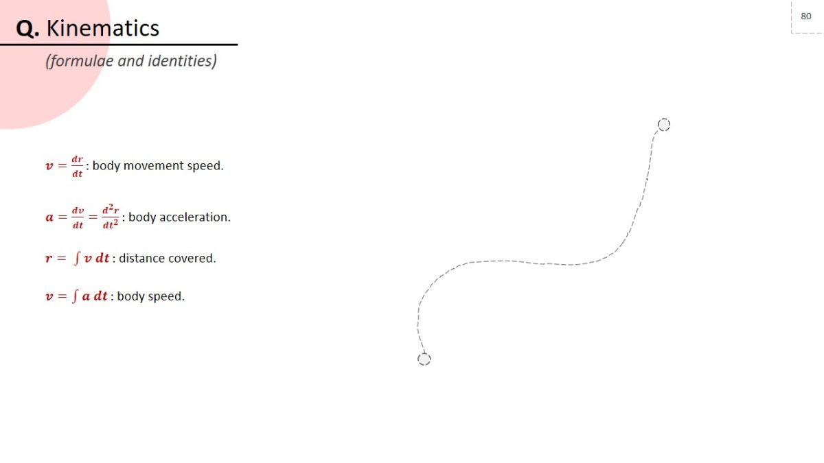
v=dr/dt: body movement speed.

a=dv/dt=(d^2 r)/(dt^2 ): body acceleration.

r= ∫υ dt: distance covered.

v=∫ a dt: body speed.

Content objectives

1. Use terminology and the language of kinematics.
2. Be able to interpret kinematic graphs for movement in a straight line.
3. Enter a vector expression, display formulas oneself for constant acceleration.
4. Use known formulas.
5. Simulate movement in the vertical plane under the action of gravity.

Example

Assignment:

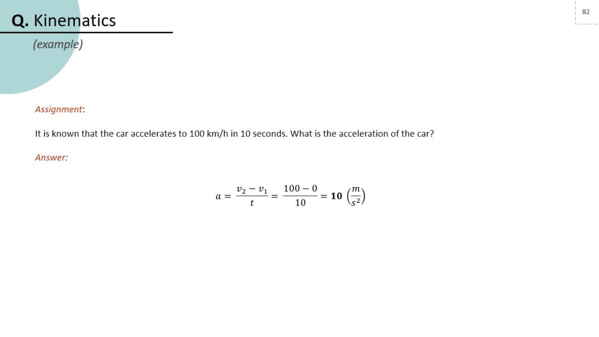
It is known that the car accelerates to 100 km/h in 10 seconds. What is the acceleration of the car?

Answer:

a= (v_2-v_1)/t= (100-0)/10=10 (m/s^2 )

Forces and Newton’s laws

Notation

• F : Force or resultant force.
• N : newton.
• Nm: newton metre.
• m: mass of an object.
• a: acceleration.
• µ: coefficient of friction.

Formulae and identities

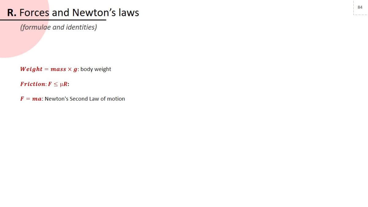
Weight=mass×g: body weight.

Friction:F≤µR:

F=ma: Newton’s Second Law of motion.

Content objectives

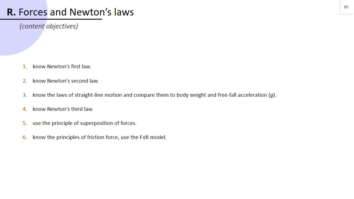
1. Know Newton’s first law.
2. Know Newton’s second law.
3. Know the laws of straight-line motion and compare them to body weight and free-fall acceleration (g).
4. Know Newton’s third law.
5. Use the principle of superposition of forces.
6. Know the principles of friction force, use the F≤R model.

Example

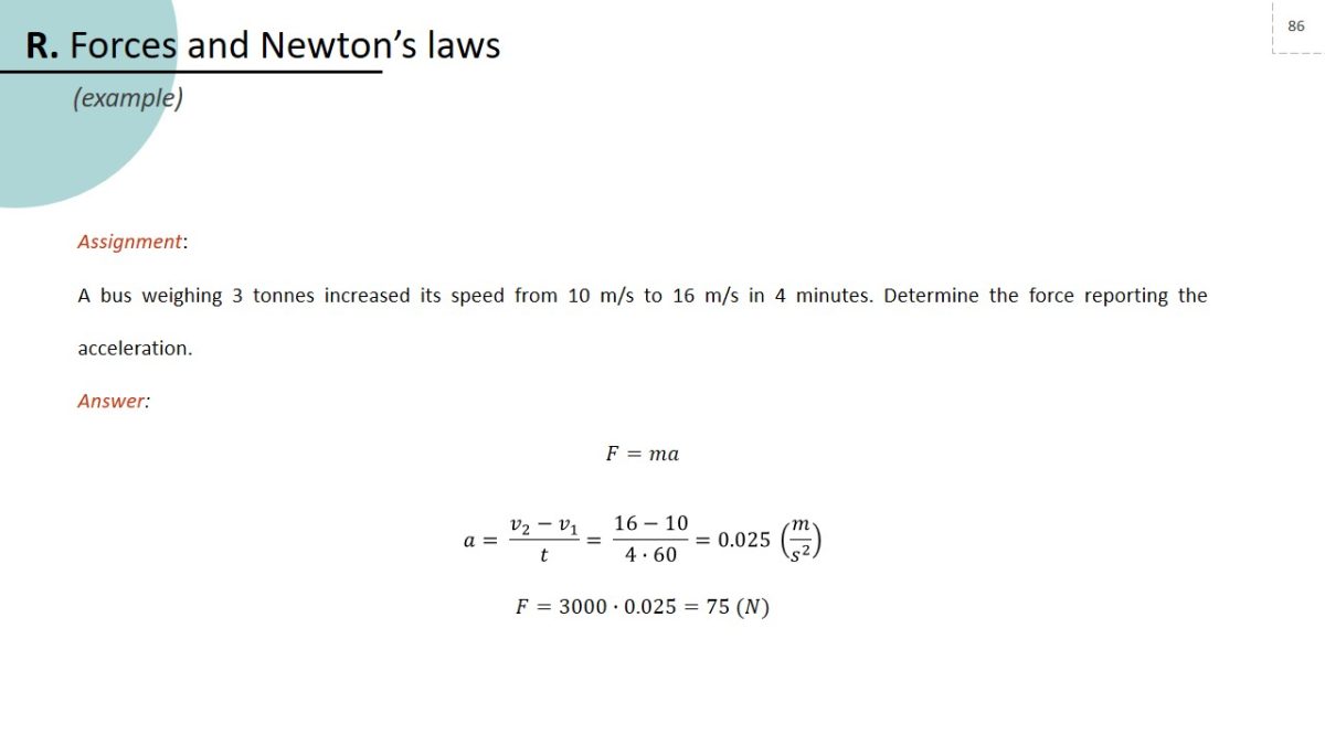
Assignment:

A bus weighing 3 tonnes increased its speed from 10 m/s to 16 m/s in 4 minutes. Determine the force reporting the acceleration.

Answer:

F=ma.

a= (v_2-v_1)/t= (16-10)/(4∙60)=0.025 (m/s^2 )

F=3000∙0.025=75 (N).

Moments

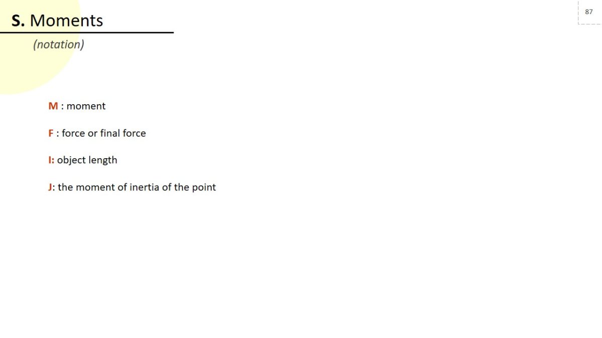
Notation

• M : moment.
• F : force or final force.
• I: object length.
• J: the moment of inertia of the point.

Formulae and identities

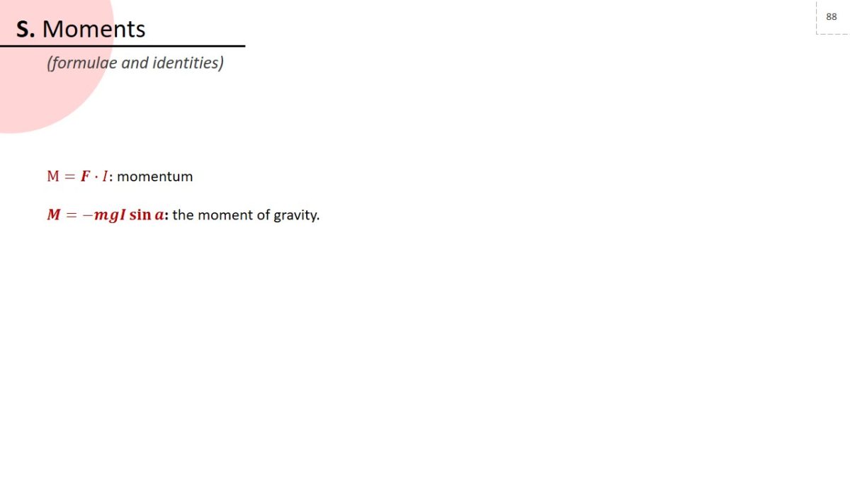
M=F∙I: momentum.

M=-mg I sin⁡ a: the moment of gravity.

Content objectives

Use the moment model in static terms.

Example

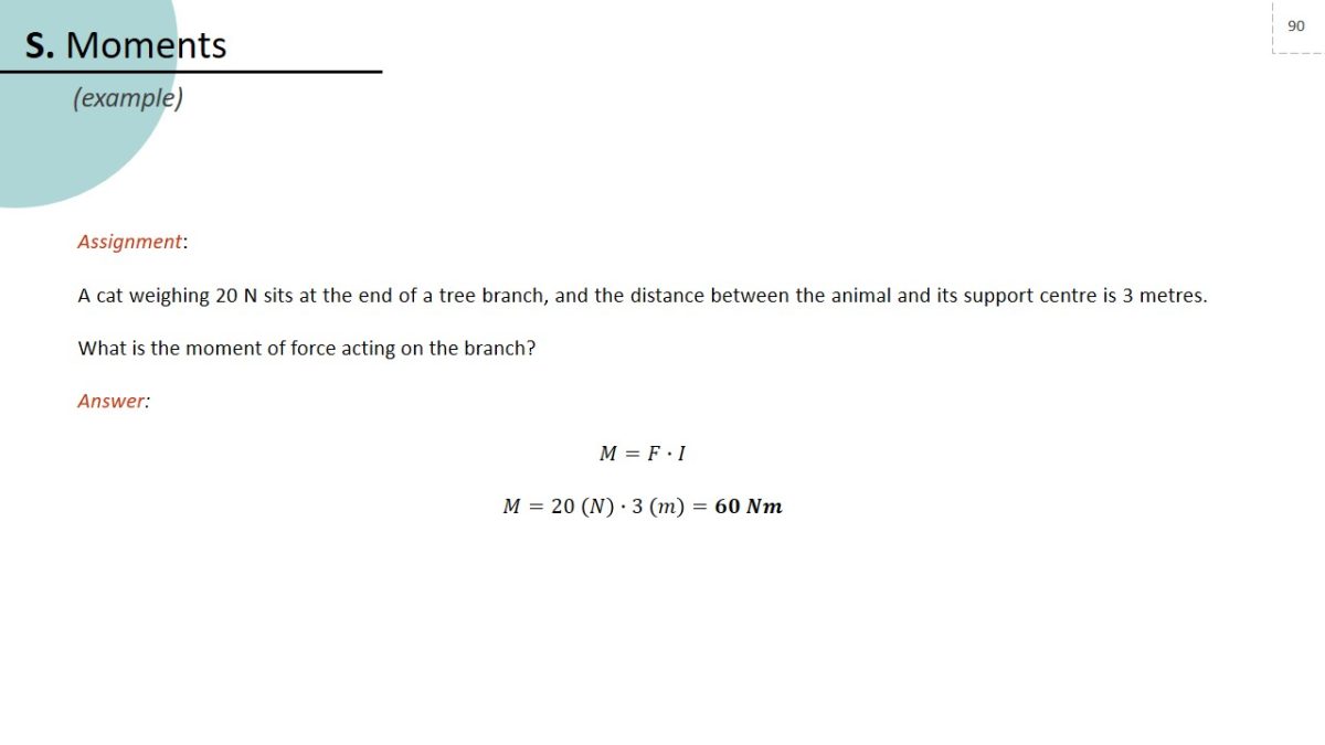
Assignment:

A cat weighing 20 N sits at the end of a tree branch, and the distance between the animal and its support centre is 3 metres. What is the moment of force acting on the branch?

Answer:

M=F∙I

M=20 (N)∙3 (m)=60 Nm.