Introduction
In everyday life, ship towing is used to move heavy cargo vessels using more active smaller ships that drag an object by applying force. Reasons for such towing may be, for example, shallow water that makes a large ship unable to engage its engines or a breakdown that results in an inability to continue the route (Whiteford, 2021). In this process, it is essential to consider the aerodynamic characteristics of the process, which are relevant to enhance the effects of towing. For example, if the velocity of the vessel is too high, the object may get stuck in curves or crash into other objects in traffic while being manipulated. In order to increase the effects of towing, it is necessary to conduct tests in which the process is studied beforehand.
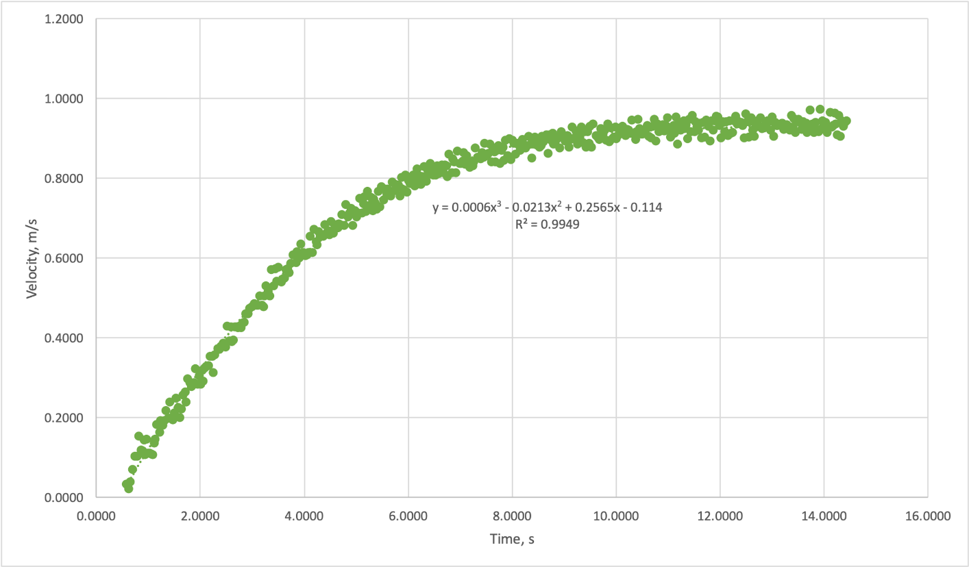
In this research report, such a towing process is the basis for the experiment. A small Rough Hull-type ship weighing 1.65 kg was placed in a pool of water, and a cable was attached to the front edge of the vessel. The tension of this rope caused a force that caused the Rough Hull to move forward along the central axis of the pool. This movement caused the water to be perturbed, which gained velocity as it emerged from its resting state. It was the velocity of the water that was measured in this work with digital sensors and recorded. In addition, the resistances exerted by the ship against the motion were to be measured. A total of five tests were conducted, of which the second was used as the one of most significant interest. In particular, the dependence curve in this test (see figure below) was as smooth as possible and had no significant outliers. The data were processed by removing the left and right edges in the sample so as not to cause significant distortion for the regression analysis. The use of MS Excel was necessary to perform mathematical analysis, construct graphical visualizations, and verify the accuracy of the manually obtained responses.
Results and Discussion
The data from the second test
In the first part of this work, the data from the second test, obtained after cutting off the extreme ends, were loaded into MS Excel and sorted in order of increasing time values. To identify the relationship between the variables of velocity (dependent variable) and time (independent variable), the data were plotted on a scatter plot as shown in the figure below. As can be seen from the graph below, the velocity did not increase linearly with time but had a different form of dependence. During the first six seconds, there is some growth, probably linear, but then the function comes to a nearly horizontal line where the velocity does not change significantly. In this state, the acceleration of such a function appears to be minimal because there is no meaningful change in velocity over time.

The same figure shows the regression curve equation that best fits the data. Specifically, the regression offers a third-degree polynomial function, that is, a cubic polynomial that describes the behavior of velocity over time (CueMath, 2020). The measure of this fit is the coefficient of determination, which for this model is 0.9949. Of course, MS Excel offers the possibility to increase the degree of the polynomial, but this does not significantly affect the growth of R2 but significantly complicates the calculations. Therefore, the following entry is optimal for use as a function of velocity on time:
If we take the derivative for this function, it is possible to determine the expression for acceleration because, as mentioned earlier, acceleration is the change in velocity over time, as follows from the physical meaning of this quantity:
The resulting record for acceleration can be used to calculate the value of real acceleration of the Rough Hull ship model at different times. For example, when the time was zero, the acceleration was:
Certainly, this answer does not make physical sense, since at time zero Rough Hull was not moving, and hence no acceleration was observed. However, this is an excellent demonstration of some assumption that must be made when using regression analysis: the y-intercept of a function does not always make physical sense.
At the same time, if we conduct integration for the velocity function, it becomes possible to go in the direction of increasing the degree of the original polynomial, that is, to find an antiderivative. Without integration bounds, in the case of an indefinite integral, the product of such a calculation contains the constant C. However, when the integration bounds are set, the constant is omitted, and it becomes possible to find the specific value of the area of the figure that is formed between the curve and the X-axis. The integration bounds for this calculation will be the time values from zero when the test was started to the maximum time value in the sample, viz.:
From the calculations, it follows that the ship covered a distance of 10.2 meters during the first 14.4239 seconds. Indeed, this answer is approximate since rounding was used for the calculations. In addition, we have hand-cut some of the data, and it is likely that single valuable points were lost, which may have affected the final result. Nevertheless, it gives a good indication of how far the ship actually approximately advanced during the test. For all five tests in which the same force was applied to the ship, the velocity functions behaved in an analogous manner. If the test times were identical, then it can be stated with a certain margin of error that the Rough Hull went about the same distance of 10.2 meters.
The maximum values that the ship reached
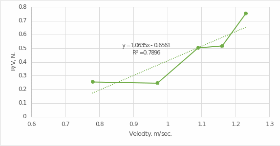
The test also measured the maximum values that the ship reached in each of the five tests, as well as the drag resistance. Resistance divided by velocity gave the variable R/V, which determined the relationship between the variables. For the purposes of the current section, a regression analysis was performed between V and R/V to answer the question of whether the relationship between the variables was linear. It is expected that under zero velocity conditions, there was no drag, the ship was not actually moving. The table below reports the results of the measurements and provides information on the calculations performed in Excel for future reference.
At first glance, we can see that with increasing velocity, there was an increase in R/V as well. However, this information is not enough to qualitatively evaluate the nature of the relationship. Instead, we must first calculate the correlation coefficient to determine the strength and direction of the relationship between the variables.

This indicates that there is a strong positive correlation between R/V and V. The square of this value leads to the coefficient of determination as a measure of the reliability of the regression line:
This is not a very high value, but still a reliable indicator for the regression model. The regression equation itself has the following form:
In which m defines the slope coefficient and b is the y-intercept of the function. Recall that since the relationship between the variables is predicted to be directly proportional, and given their physical meaning, the slope is expected to be positive and the y-intercept to be zero (Bevans, 2022). This is easy to check because the slope value can be calculated manually as follows:

And to calculate the y-intercept, we can use the following formula:

The regression equation is as follows:
The resulting value should be compared to the results of the automatic Excel calculations to determine the quality and reliability of the results. In particular, the figure below shows a regression straight line for this data set, with the equation indicated. As this figure shows, the equation obtained above is generally consistent with what was done in Excel. In other words, there are no significant deviations between the two equations, and any errors are due to statistical calculation error.

The SNR level
For the third part of this report, it was necessary to calculate the SNR level, which determines the purity and quality of the signal. In telecommunications technology, the SNR parameter characterizes the ability to separate the useful signal from noise. Sources of such noise can be external interference, thermal and mechanical fluctuations, electromagnetic distortions, and other factors that affect the quality of the transmitted signal (Baker, 2020). The lower the influence of such noise, the more efficiently the signal is transmitted between points, which is a key need in telecommunications. For the current section, the SNR was calculated for fifteen randomly selected data points that had close to the maximum rate. These data points are shown in the table below:
To determine the SNR, we need to know the actual ratio of the mean value of the function to its standard deviation:
Excel allows us to quickly calculate these values using the corresponding functions =AVERAGE() and =STDEV.S(). Then we can substitute the known values in the formula:
The resulting value defines an elevated level of SNR, which means that this function can be used to design signal transmission and is generally of high reliability.
Mathematical calculations for the ship’s velocity function
In the last part of the report, it is necessary to make mathematical calculations for the ship’s velocity function:
The calculations involve the operations of differentiation and double differentiation, in order to find entries for velocity and acceleration respectively:
The velocity will be zero at the next moment:
Another time value, the second root of the quadratic equation, was negative, which made no physical sense. The acceleration would be zero at the time:
Six seconds later, the speed was equal to:
Four seconds later, the acceleration was:
Finally, after ten seconds, the ship went the following distance:
Conclusion
In conclusion, it is worth noting that modeling is used to deeply explore the relationship between variables and predict their values. In this paper, mathematical manipulation was applied to the second test, in which the Rough Hull was pulled along the main axis of the basin with some force. The following key conclusions were drawn:
- Velocity is nonlinearly dependent on time.
- The equation for the dependence of velocity on time has the form:

- SNR, as a measure of signal purity, was high and equal to 52.33
- R/V as a function of V had a linear relationship, and the results of the calculations corresponded well with the automatic Excel calculations.
As a general corollary, this work can be considered a success, and the findings can be used to further design the Rough Hull tow.
Reference List
Baker, A. (2020) What is SNR and how does it affect your signal? Web.
Bevans, R. (2022) Simple linear regression | an easy introduction & examples. Web.
CueMath (2020) Cubic polynomial. Web.
Whiteford, S. (2021) How do tugboats work? Web.
Appendix A
Direct Measurement Data Resistance and Velocity for the Data
