Independent T-Test
The statistical test
Independent t-test.
The Problem
The student t-test is a parametric test, which implies that the sampling distribution should be normal and the variances should be equal (Field, 2013; Warner, 2012). This question aims to determine whether wearing an invisibility coat (independent variable) determines the incidence of mischievous acts (dependent variable).
Research question
Does the number of mischievous acts increase when an invisibility cloak is worn compared to when the cloak is not worn?
The hypotheses
The null hypothesis is that the means of mischievous acts in people wearing the invisibility cloak and those without the invisibility cloak are equal: H0: u1 = u2. The alternate hypothesis is that the means of mischievous acts in the two groups are not equivalent: HA: u1 ≠ u2.
Findings
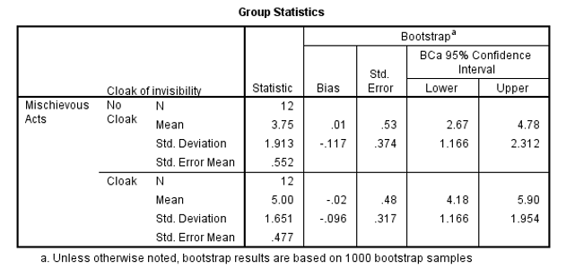
Output 1 shows the group statistics for each category. There were 12 participants in each group as indicated by the row labeled N. The average number of mischievous acts for the group that did not have the invisibility cloak was 3.75. This group had a standard deviation of 1.913 and a standard error of 0.552. The bootstrap standard error estimate was 0.53 with a confidence interval of the means ranging from 2.92 to 4.58. The standard error of means was estimated by finding the quotient of the standard deviation and the square root of N (Carlson & Winquist, 2017).
SE = 1.913/√12
= 1.913/3.464
= 0.552.
On the other hand, the group with the invisibility cloak reported an average of 5 mischievous acts, a standard deviation of 1.651, and a standard error of 0.477.
The bootstrap standard error reduced to 0.46, and the range of the confidence interval for the mean was from 4.33 to 5.67. Comparing the confidence intervals of the two groups showed an overlap, which insinuates that the two groups may be from the same population (Jackson, 2012).
Output 2 shows Levene’s test, which indicates whether the variances are equal or unequal. When Levene’s test yields a significant outcome (at p values less than 0.05), the variances are unequal, which violates the law of homogeneity (Carlson & Winquist, 2017). In such a case, the value of t when equal variances are not assumed should be used in Output 3. In this case, Levene’s test was insignificant (p= 0.101). Therefore, it was correct to assume that the variances between the groups were equal.
The overall finding was that subjects who received the invisibility cloak engaged more in mischievous acts (Mean = 5, Standard error = 0.48), than those who did not wear the cloak (M = 3.75, SE = 0.55). This difference, −1.25, BCa 95% CI [−2.695, 0.070], was not significant t(22) = −1.71, p =.101. To determine the significance of the impact of the cloaks (-1.25), the following calculation was done:
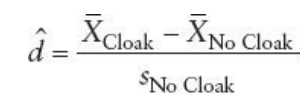
d= (5-3.75)/1.91
d= 0.65.
This value shows that there was 0.65 of a standard deviation disparity between the two groups concerning their engagement in mischievous behavior. Therefore, as much as the effect of the invisibility cloak was not statistically significant, its impact on mischievous behavior was 0.65.


Dependent T-Test
The statistical test
Dependent t-test.
The Problem
The aim of the question is to determine whether wearing an invisibility coat (independent variable) influences the extent of mischievous acts (dependent variable).
Research question
Does the data suggest that mischievous acts are significantly more when one is wearing an invisibility cloak than when one is without the cloak?
The hypotheses
The null hypothesis is that the mean difference of mischievous acts between cloak and no cloak is zero. H0: µ1 – µ2 = 0. The alternate hypothesis is that the mean difference of mischievous acts between people wearing the invisibility cloak and those without the cloak is not zero. HA: µ1 – µ2 ≠ 0.
Findings
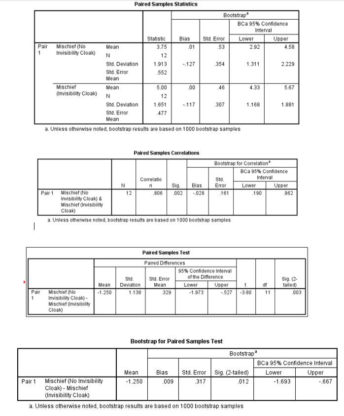
Overall, participants that received the cloak of invisibility took part in more acts of mischief (M = 5, SE = 0.477), than those who did not receive the cloak (M = 3.75, SE = 0.552). This difference, −1.25, BCa 95% CI [−1.693, −0.667], was significant t(11) = −3.80, p = 0.003. It also represented a medium sized effect of d = 0.65.
Application of T-Tests on the Research Problem
Problem 1
What form of training is more effective in the training of staff members on the utilization of the equipment? Why?
The statistical test
Independent t-test.
The Problem
The requirement of the problem is to determine the intervention that led to the highest utilization of equipment among the employees.
Research question
Is the utilization of equipment in employees taught by intensive classroom training better than those who have undergone hands-on training?
The hypotheses
The null hypothesis is that the means of the willingness to use equipment between people trained by intensive classroom training and hands-on training are equal: H0: u1 = u2. The alternate hypothesis is that the means of willingness to use equipment between people trained by intensive classroom training and hands-on training are not equal: HA: u1 ≠ u2.
Findings
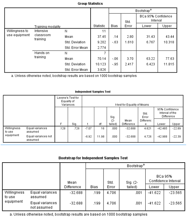
There was a higher mean usage of equipment for individuals that received hands-on training (70.14, SE= 3.826) than those who received intensive classroom training (37.45, SE= 2.774). This difference -32.688, BCa 95% CI [-41.622, -22.565], was significant t(11.98) = −6.92, p ˂ 0.001.
Problem 2
How does the intervention correlate with the frequency of the use of technology, patients’ satisfaction, as well as the quality of services provided?
The statistical test
Paired t-tests.
The Problem
The problem aims at comparing four different means. However, the student t-test is only applicable when comparing two means. Therefore, three different tests were done to compare the intervention (training) and the frequency of the use of technology, patients’ satisfaction, and the quality of services provided.
Research question 1
Is the frequency of technology use higher when staff are trained through intensive classwork instruction than through hands-on training?
The hypotheses
The null hypothesis is that the mean difference of the frequency of technology use between employees who received intensive classwork training and those who underwent hands-on training is zero. H0: µ1 – µ2 = 0. The alternate hypothesis is that the mean difference of the frequency of technology use between intensive classwork and hands-on training is not zero. HA: µ1 – µ2 ≠ 0.
Findings
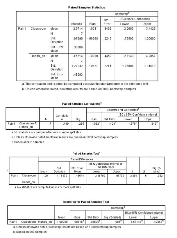
Overall, the frequency of technology use was higher among employees who received hands-on training (M = 3.57, SE = 0.48), than intensive classwork instruction (M = 2.57, SE = 0.37). This difference, −1.25, BCa 95% CI [−1.571, −0.429], was not significant t(6) = −2.291, p = 0.062.
Research question 2
Is patient satisfaction higher when workers are trained through intensive classwork instruction than hands-on training?
The hypotheses
The null hypothesis is H0: µ1 – µ2 = 0, whereas the alternate hypothesis is HA: µ1 – µ2 ≠ 0.
Findings
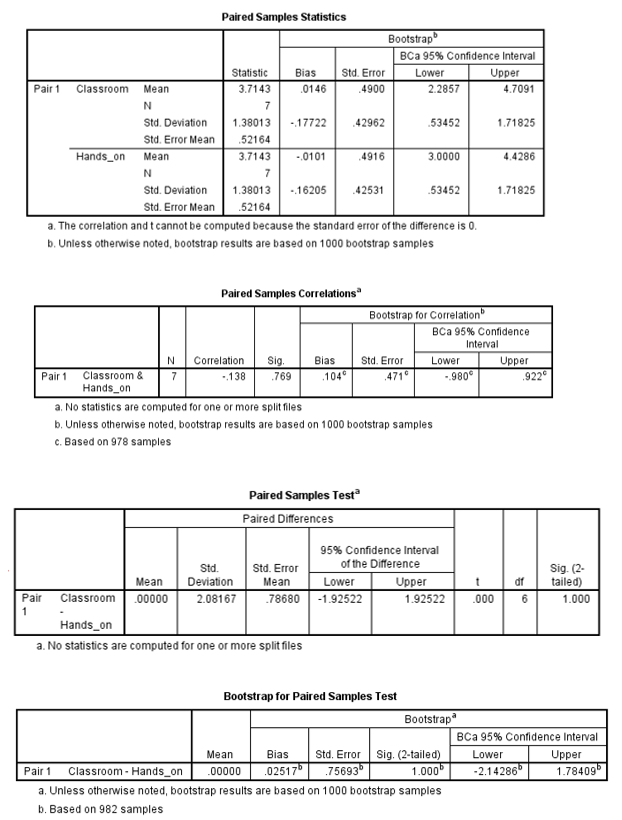
There was no difference in patient satisfaction between employees who received hands-on training (M = 3.71, SE = 0.4621) and those who received intensive classroom instruction (M = 3.71, SE = 0.4621). This difference, 0.00, BCa 95% CI [−2.141, 1.784], was not significant t(6) = 0.00, p = 1.
Research Question 3
Is the quality of services higher when employees are trained through intensive classwork instruction as opposed to hands-on training?
The hypotheses
The null hypothesis is H0: µ1 – µ2 = 0, whereas the alternate hypothesis is H1: µ1 – µ2 ≠ 0.
Findings
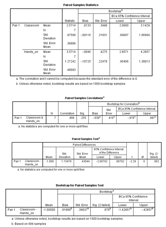
It was observed that the quality of services was higher among employees who received hands-on training (M = 3.571, SE = 0.48) than those who received intensive classroom instruction (M = 2.571, SE = 0.37). This difference, 1.0, BCa 95% CI [−1.428, 0.428], was not significant t(6) = -2.29, p = 0.062.
Problem 3
How does the intervention affect the participants’ willingness to implement their own research or find new ways of utilizing the equipment?
The statistical test
Paired t-test.
The Problem
This problem requires the comparison of three means: the intervention, willingness to implement their own research, and finding new ways of utilizing equipment. Therefore, given the limitation of the t-test in comparing means, only two means can be compared at any given time (Terrell, 2012; Ross, 2014).
Research question 1
Is the willingness to implement own research high when employees are trained through intensive classwork instruction as opposed to hands-on training?
The hypotheses
The null hypothesis is H0: µ1 – µ2 = 0, whereas the alternate hypothesis is HA: µ1 – µ2 ≠ 0.
Findings
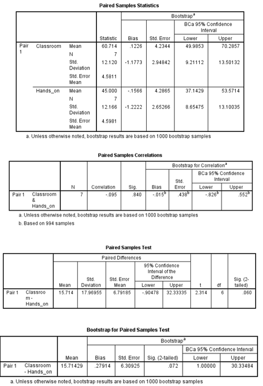
It was observed that the willingness to implement own research was higher among employees who received intensive classroom training (M = 60.714, SE = 4.581) than those who received hands-on training (M = 45.000, SE = 4.598). This difference, 15.714, BCa 95% CI [1.000, 30.334], was not significant t(6) = 2.314, p = 0.060.
Research question 2
Is the capacity to find new ways of utilizing equipment higher when employees are trained through intensive classwork instruction than when trained through a hands-on curriculum?
The hypotheses
The null hypothesis is H0: µ1 – µ2 = 0, whereas the alternate hypothesis is H1: µ1 – µ2 ≠ 0.
Findings
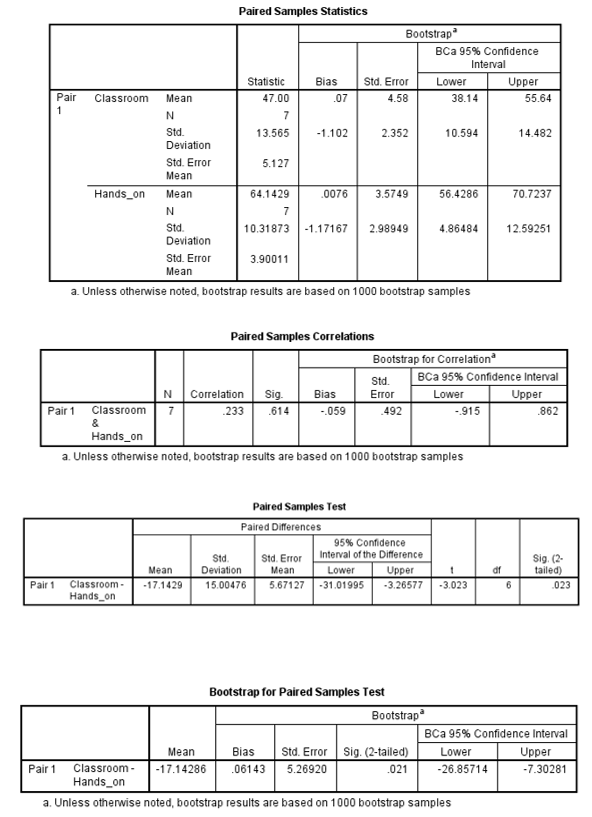
The capacity to find new ways of utilizing research was higher among employees who received hands-on training (M = 64.143, SE =3.900), than those who received intensive classroom training (M = 47.007, SE = 5.127). This difference, -17.143, BCa 95% CI [-26.857, -7.3028], was significant t(6) = -3.023, p = 0.023.
Problem 4
How does the intervention affect the participants’ willingness to affect the hospital’s performance as well as certain purchasing policies?
The statistical test
Independent t-test.
The Problem
The requirement is to compare the impact of the intervention on employees’ willingness to affect the hospital’s performance as well as certain purchasing policies.
Research question
Is the capacity to affect the hospitals’ performance higher when workers receive intensive classwork instruction than when they receive hands-on training?
The hypotheses
The null hypothesis is H0: µ1 – µ2 = 0, whereas the alternate hypothesis is HA: µ1 – µ2 ≠ 0.
Findings
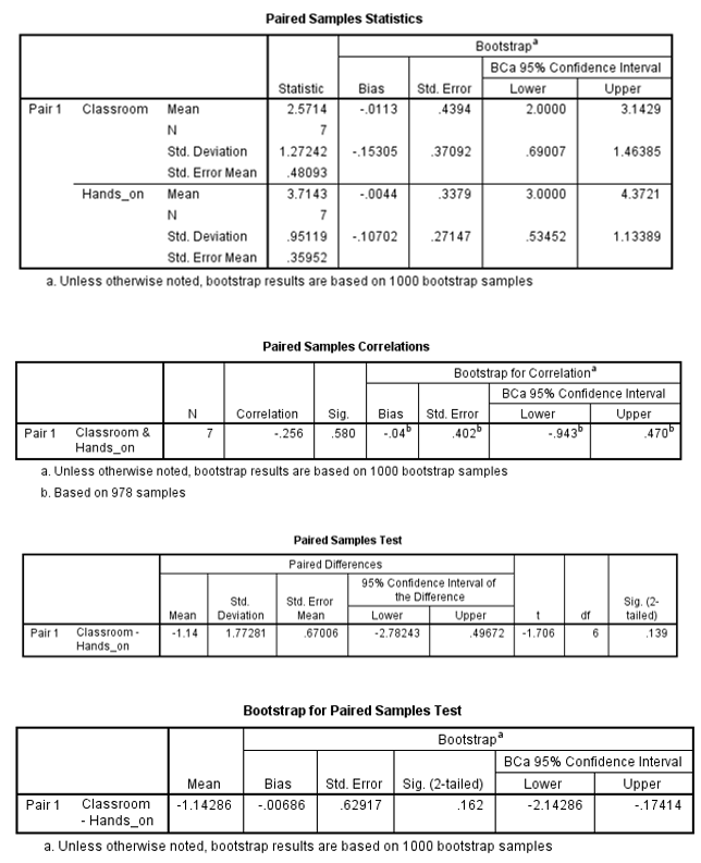
The capacity to affect the hospitals’ performance was higher among employees who received hands-on training (M = 3.714, SE = 0.359) than those who received intensive classroom training (M = 2.571, SE = 0.481). This difference, -1.1429, BCa 95% CI [-2.1429, -0.1741], was not significant t(6) = -1.706, p = 0.139.
References
Carlson, K. A., & Winquist, J. R. (2017). An introduction to statistics: An active learning approach. Los Angeles, CA: Sage Publications.
Field, A. P. (2013). Discovering statistics using IBM SPSS statistics. Web.
Jackson, S. J. (2012). Research methods and statistics: A critical thinking approach (4th ed.). Belmont, CA: Cengage Learning.
Ross, S. M. (2014). Introduction to probability and statistics for engineers and scientists (5th ed.). San Diego, CA: Academic Press.
Terrell, S. R. (2012). Statistics translated: A step-by-step guide to analyzing and interpreting data. New York, NY: Guilford Press.
Warner, R. M. (2012). Applied statistics: From bivariate through multivariate techniques: From bivariate through multivariate techniques (2nd ed.). New Delhi, India: Sage Publishers.