Introduction
There has long been established a link between women’s participation in paid labor and the division of chores between partners at home. Women who participate in paid work have less time and have the economic wherewithal to hire help; therefore, they experience less in household work.
In theory, there are words such as “time availability” and “specialization” which intersect with others, such as “relative resources” and “time availability”; these are variables that distill to a trade-off between unpaid and paid work (Mendiola et al., 2017, pp. 42–62). The decision to engage in either could stem from rational economic decisions between partners or from a negotiation based on available resources. The essence of this revelation is that women’s financial independence is a crucial factor in determining the division of chores in the home.
This paper will focus on the factors affecting the division of chores in the home. The dependent variable in the study is the number of hours spent on housework per week. One independent factor that will be investigated includes years of full-time education completed. It has been established that women’s economic independence affects their availability for chores; interestingly, studies show that women breadwinners still do more house chores (Mendiola et al., 2017, pp. 42–62). Another factor that will be investigated is the number of children living at home. It is natural to expect the number of children to be directly correlated with the amount of work available in the house. Since it has been established that the labor situation culminates in a rational agreement most of the time, one would expect one of the parents to remain at home to take care of children.
Marital status will also be investigated as an independent factor given that unmarried people have nobody to negotiate with and have fewer children and fewer resources. However, this experiment goes a step further to make the legality of the marital status a variable. According to Cerrato and Cifre (2018, pp 1330), women do more housework than men; however, this pattern is most prevalent among married. Women in spousal relationships spend more time on household chores than those in de facto relationships. Employment relations will also be analyzed as an independent variable. There’s no doubt that the type of employment affects the resources available, which in turn affects the negotiation on who will do the labor.
One would expect a self-employed person to reap the benefits that come with autonomy. A recent study revealed that working from home or freelancing leads to women shouldering a more significant proportion of household chores (Del Boca et al., 2020, pp 1001-1017). Correlation and regression analyses will be conducted on these variables. The dependent variable is the number of hours in a week spent on household chores. Stepwise regression will be used to try different blocks of variables to check their cumulative effect on the dependent variable’s variability. Even after incrementally adding other variables, gender was the most critical factor in predicting labor division in the home.
Methods
The data for this report is obtained from the European Social Survey (ESS) 2010 round 5. The ESS survey is a European endeavor to collect data about the attitudes, behavior, and beliefs patterns of the different populations of Europe. The ESS survey specification details the responsibilities and tasks for each round of the survey. The specification’s main points are preparation of the questionnaire, data collection preparation, sampling, data collection process, and data processing.
The survey source questionnaire consists of two sections, the rotating section, and the core section. The core module is aimed at a time-series collection of data to capture changing attitudes in Europe, while the 11 rotating modules are chosen after an open call for proposals (European Social Survey, n.d.). Some of the rotating modules cover such topics as gender, social inequalities, values of democracy, digital social contacts, justice and fairness, the timing of life, attitudes to climate change, welfare attitudes, and immigration (European Social Survey, n.d.). It also covers social health inequalities, personal and social well-being, work and family well-being, ageism, trust in the criminal justice system, and citizenship involvement in democracy.
The ESS sampling plan is to achieve workable and equivalent objectives for all the participant countries. The samples are required to be representative of all people above 15 years who are residents in the countries regardless of nationality, language, or citizenship (European Social Survey, n.d.). Persons are selected using a random probability mechanism on every level. Sometimes, sampling frames of persons, households, or addresses are used. Every country’s aim is a sample size of 1500 or 800 if the ESS country has a population of less than 2 million (European Social Survey, n.d.). Quota sampling is disallowed at all stages. It is also not allowed to substitute for non-responding individuals or households.
Data collection is done through CAPI face-to-face interviews in all participant countries. In each country, a standard is followed, which includes a response rate target of 70%, a maximum of 3% noncontact rate, fieldwork period of a minimum of 6 weeks within the survey period of 5 months (Vandenplas and Loosveldt, 2017, pp 212-232). Face-to-face briefing of interviewers is also required, and each interviewer’s maximum workload is 48 samples (European Social Survey, n.d.). Interviewers are supposed to have a maximum of 4 contact attempt calls, with at least one during the weekend and one in the evening (Vandenplas and Loosveldt, 2017, pp 212-232). The interviewers are supposed to have contact forms in the field, conduct back checks for close monitoring of the process.
The ESS 2010 round 5 dataset has 674 variables with 52458 total observations (European Social Survey, n.d.). Out of these 674, this report is concerned with hwwkhs (total weekly hours one spends on housework), gender(gndr), and (years of full-time education completed(eduyrs). The others are children living at home or not(chldhm), the legality of marital status (maritalb) and employment relation(emplrel) (European Social Survey, n.d.). The emplrel variable was recoded into abc_1 for employee, abc_2 for self-employed, abc_3 for working from home, abc_4 for not applicable, abc_5 for refusal, abc_6 for “don’t know,” and abc_7 for no answer.
The maritalb variable was split into the variables b_1 for legally married, b_2 for in a legally registered union, b_3 for legally separated, b_4 for legally divorced, b_5 for widowed/civil partner, b_6 for none of the above, b_7 for refusal. Furthermore, it was split into b_8 for don’t know and b_9 for no answer. The variable gndr was recoded into u_1 for male and u_2 for female, and u_3 for no response. On the other hand, the variable chldhm was split into uu_1 for respondent lives with children, uu_2 for ‘does not live with children,” and uu_3 for not available. The recording of the variables was necessary to augment the composite variables.
Results
Correlation Analysis
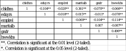
In table 1 above, considering the dependent variable hwwkhs only, it can be seen that it relates significantly with chldhm at a rate of -0.006, which is very low, almost negligible. It correlates considerably with eduyrs at a low negative rate of -0.076; it also correlates significantly with emplrel though the rate at a negative rate of -0.114. maritalb, on the other hand, had a significant negative correlation with hwwkhs at a low rate of -0.087. Finally, gndr had a significant correlation with a moderate positive correlation.
Regression Analysis
Stepwise regression was used to test how much the independent variables affected the dependent variable. The most significant variable in predicting the weekly hours spent in housework was gender. It will become evident that the addition of other variables in the stepwise regression does not increase the predictive power over gender. Moreover, most variables will be rejected for failing the multicollinearity test. Model 1 summary was F(1, 27997)= 6014.554, p<0.01, R2adj =.177. The dependent variable was hwwkhs, while the independent variable was male gender (u_1). The coefficient for the independent variable was -11.872, indicating a negative gradient of a regression line. The male gender explains 17.7% of the variability of the dependent variable.
The second model added years of full-time education on top of the u_1 male gender variable. The model summary was F (2, 27993) = 3187.55, p<0.01, R2adj =.187. After adding the second variable, adjusted R-Square was 0.187, meaning that the two independent variables could now explain 18.7% of the dependent variable instead of 17.7%. The variable had a standardized Beta coefficient of -0.097, which is low. The variable was not included in the final model because of collinearity testing.
The third regression model added the variables b_1(marital status legally married), b_2(in a legally registered union), b_3( maritalb = legally separated), b_4( maritalb = legally divorced) and b_5(maritalb = none of the above). After adding the above variables, the model’s predictive power jumped to 0.188 in adjusted R-square. The model only showed a minor bump in predictive power. On the coefficient table, b_2 and b_3 were not significant predictors. However, all the maritalb variables were excluded from the model for multicollinearity.
The third model added the variables uu_1 (chldhm = respondent lives with children at home). The model’s summary was F (2, 27998) = 3073.39, p<0.01, R2adj =.180. These details show that the added variable did not add considerable predictive power to the model. The variable was excluded from the model for failing the assumptions test. The fourth model added abc_2 (emplrel= self-employed) and abc_3(emplrel = working for own family business). The model’s summary was F (3, 27995) = 2050.26, p<0.01, R2adj =.180. The added variables did not increase the predictive power considerably. They were also excluded from the model for failing the assumptions test. The fifth model included all the above variables (u_1, b_2, b_3, b_5, abc_3, b_4, Years of full-time education completed, uu_1, abc_2, b_1) into the model. After inclusion of the additional variables, the model’s summary was F (10, 27785) = 709.24, p<0.01, R2adj =.203. The additional variables gave the prediction power a boost to 20.3% from 17.7%; still, all were excluded for failing the assumption test.
Discussion
The correlation results indicate that total weekly hours spent doing housework are inversely correlated with the number of years spent in full-time education. It also increases with legal marital status and with the female gender. Moreover, children at home also seem to correlate with the dependent variable positively. The first regression model had only one independent variable – gender- which showed an inverse correlation with quite a considerable prediction power. This observation is in line with the literature review, which shows that women spend more time doing housework than men, whether due to cultural reasons or mutual agreement between spouses.
In the second model, the variable number of years spent in education was added to the model but did not improve its predictive power. It has already been established that gender is the main predictor of the number of hours spent doing housework. The third model added “legally married” as a variable; even after adding this variable, the model only negligibly increased its predictive power. The variable was also flagged for violating the condition of multicollinearity. This observation is consistent with the literature review that shows that gender is the main predictor of weekly hours spent doing house chores.
In the third model, the variable that was added while controlling for gender was “living with children at home,” which increased the predictability by negligible amounts. The variable was also flagged for multicollinearity, meaning that it could be predicted by the other independent variables, in this case, gender. This also underscores the literature review observations that gender is the main predictor of the number of hours spent on house chores. In all the models, all the variables added were not adding more predictability to the simple linear regression with one variable. Although most would be significant predictors, they would fail in multicollinearity testing.
The weakness of the study is that the survey question may be confusing. The survey asks the interviewee how many hours they are likely to spend doing housework such as cooking, cleaning, laundry, shopping, property maintenance but excluding childcare. It seems confusing that childcare is not included as part of housework, yet children could be a causal variable for added house chores. Suggested improvement would be to have childcare in this variable since it is also a highly gendered activity that cannot be separated from the others.
Conclusion
This report aimed to investigate the factors affecting the division of labor at home with gender as the controlling variable. The correlation experiment revealed that the number of weekly hours spent on housework was significantly correlated with years spent in education, gender, number of children in the home, the legality of marriage, and employment relation. More specifically, it was determined that females are more likely to spend more hours doing housework than men. It was also discovered that the number of years spent on education had a negative effect on the number of hours spent performing house chores. Moreover, the number of children at home had a positive correlation with the hours spent performing housework. It was also determined that self-employment had a positive correlation with the dependent variable as opposed to employment. This was consistent with the literature review case where a study during the pandemic showed that freelancing and working from home led to women shouldering more housework burden.
In the regression analysis, gender was used as the controlling variable. In each iteration of the regression, variables would be added to determine their net effect on predictability power. It was determined that despite adding many variables, the net impact on the model’s predictive ability was negligible. Gender had the most predictive control over all the variables. Another salient observation from the experiment was that even the variables that had significant predictive power on the dependent variable would get flagged for autocorrelation and would end up being excluded from the models. This shows that most of the variables were also linearly related to gender. For instance, it is noted that men typically spend more time in education; this factor eliminated the model’s variable.
It has been established that women typically spend more time performing house chores. Even factors that one would intuitively think would reduce this appear not to affect this trend significantly. The results raise several practical implications regarding equality between women and men in terms of gender issues in managing the affairs in the home. Social changes happening in gender roles must affect the management of the house. It must be considered that women and men place equal importance on work and family institutions. The study underscores the point that even when external factors affect the balance of power in the family, women continue to emphasize family welfare more than men. These revelations come into play in various aspects of life, such as in the workplace. There is a possibility that gender roles at home affect workplace performance; organizations should develop human resource policies that consider work-family conflict.
Reference List
Cerrato, J. and Cifre, E. (2018) ‘Gender inequality in household chores and work-family conflict.’ Frontiers in Psychology, 9, p. 1330. Web.
Del Boca, D., Oggero, N., Profeta, P. and Rossi, M. (2020) ‘Women’s and men’s work, housework and childcare, before and during COVID-19.’ Review of Economics of the Household, 18(4), pp. 1001–1017. Web.
Mendiola, M., Mull, J., Archuleta, K. L., Klontz, B. and Torabi, F. (2017) ‘Does she think it matters who makes more? Perceived differences in types of relationship arguments among female breadwinners and non-breadwinners.’ Journal of Financial Therapy, 8(2), pp.?. Doi?
Sampling | European Social Survey (ESS) (n.d.). European Social Survey. [Online] Web.
Survey Specification | European Social Survey (ESS) (n.d.). European Social Survey. [Online] Web.
Vandenplas, C. and Loosveldt, G. (2017) ‘Modeling the weekly data collection efficiency of face-to-face surveys: six rounds of the european social survey.’ Journal of Survey Statistics and Methodology, 5(2)?, pp. 212-232. Web.