Introduction
Jensen Tire & Auto is experiencing a decline in performance. The company embarked on cost cutting strategy as a way to improve the bottom line. One cost that the company is targeting is the maintenance cost of its own machine. The two options that are available are either buying a maintenance contract for its machine or maintaining their own machine. The purchase price of the contract is estimated at $5,000 per annum. Thus, various statistical analyses will be used to evaluate the two options and recommend whether the company should purchase the contract or not.
Analysis
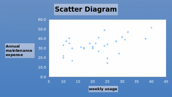
Chart 1 shows the scatter diagram for annual maintenance expense and weekly usage. The points on the diagram tend to slope upwards. This implies that there is a positive linear relationship between the two variables. Regression results are contained in Table 1. The results show that there is a weak positive correlation (0.4551) between the two variables. It implies that they move in the same direction. Thus, if one variable increases, then the other variable will also increase. Since there is only one explanatory variable, a simple regression model will be used. The regression equation will take the form presented below.
Y = a + bX
Where;
Y = annual maintenance expense
X = usage hours
Based on the results, the regression equation will be Y = 22.47 + 0.496X. The intercept value of 22.47 has no significant economic interpretation. It captures the omitted variables. The coefficient value is +0.496. The sign shows that there is a positive relationship between annual maintenance expense and the weekly usage. The value of 0.496 is the amount by which the annual maintenance expense will increase if weekly usage increases by one unit. The value of the coefficient of determination (R-square), a measure of goodness of fit, is 0.2071. It implies that the weekly usage explains only 0.2071 of the variations in annual maintenance expenses. Thus, weekly usage is a weak explanatory variable.
The significance of the explanatory variable can be evaluated using t-test. The t-statistics for weekly usage is 2.7047, while the corresponding p-value is 0.0115. The p-value is less than the significance level of 0.05. It implies that weekly usage is a significant determinant of annual maintenance expense. The results of ANOVA will be used to analyze the significance of the overall regression line. The F-statistic is 7.32, while significance F is 0.0115. This value is lower than the significance level of 0.05. This implies that the overall regression line is significant at the 95% confidence level. Thus, the regression is significant and can be used for further analysis (Black 141).
The calculations of confidence interval show that there is a 95% chance that the annual maintenance fees will fall between 2,990 and 3,640. The contract price of 5,000 is higher than the upper limit of the annual maintenance fees. Therefore, purchasing the contract will be expensive (Fraser 239).
Recommendations
The company should not purchase the contract because it will be more expensive than the current arrangement. Secondly, the weekly usage hours do not explain significant variations in annual maintenance fees. Therefore, other cost drivers such as machine hours can be used to estimate the fees.

Table 1: Regression Output.
Confidence and Prediction Interval
Average annual maintenance fee = 3,310
95% confidence interval corresponds to 5% alpha
= Ẋ ± Zs√n
= 33.1 ± 3.24
Upper limit = 3,640
Lower limit = 2,990
2,990 ≤ Ẋ ≤ 3,640
Works Cited
Black, Ken. Business Statistics, Binder Ready Version: For Contemporary Decision Making. John Wiley & Sons Ltd, 2013.
Fraser, Cynthia. Business Statistics for Competitive Advantage with Excel 2010: Basics, Model Building, and Cases. Springer Science and Business Media LLC, 2012.