Population and Participation Rates
The labor force of a country is determined by the population size as well as the number of people engaged in the labor market. Becker’s time allocation model is frequently used to study participation rates of households in labor market. According to Becker’s model, households combine goods and time to create utility-yielding commodities. In other words, households allot their time between consumption, production and labor market with respect to comparative advantages.
As a result, Becker’s model suggests that households are economic units that produce utility-yielding commodities. These commodities have two unique traits. For instance, some commodities are product-intensive while others are time-intensive. Product-intensive commodities (i.e. fast-food meals) require substantial quantities of goods and modest time whereas time-intensive commodities (i.e. leisure activities) require substantial amount of time and fewer goods to produce. These commodities are also substitutable during production. Therefore, it is possible to produce certain commodities using large quantity of goods and less time and vice versa.
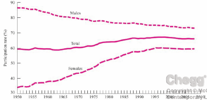
The participation rate of labor force entails comparing real labor force and potential labor force. According to Figure 1, the participation rate of males dropped gradually from 86% to 73% between 1950 and 2008. On the contrary, the participation rate of females in the labor market increased steadily during this period. The moribund participation rates among males are attributed to increased access to disability benefits, access to public and private pensions, and increase in real earnings. The increase in the participation rates for women is caused by increased marital instability, increased employment opportunities, and lower birthrates.
In addition, the participation rates among White and Black women in the labor market are almost equal. Previously, the participation rates for Black women were higher than those of White women. Conversely, the gap between the participation rates among White males and Black males have increased steadily since 1950s. For instance, the participation rates for both groups were roughly 85% in 1995. However, in 2000, the participation rate for Black males was 69% compared to 75% for White males. The difference is attributed to the limited employment opportunities for Black males compared to their White counterparts. In addition, the difference in educational achievement for both groups could explain this phenomenon.
The net impact of the added-worker effect and the discouraged-worker effect is demonstrated by the cyclic changes in participation rates. The added-worker effect lends credence to the notion that when the sole wage earner in a household loses his/her employment, other household members will seek short-term employment in the labor market to augment household income. On the other hand, the discouraged-worker effect emphasizes that unemployed workers may become unenthusiastic (especially during a recession) about securing well-paying jobs such that they may stop looking for job opportunities in the labor market.
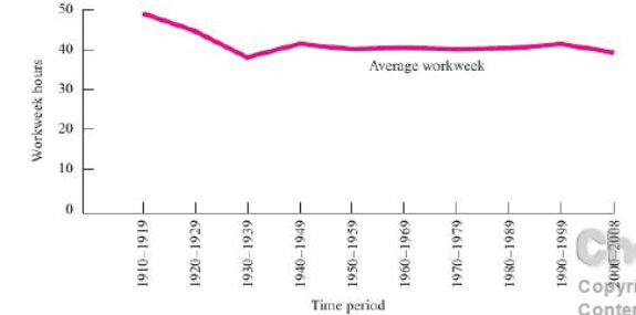
Finally, Kniesner posits that educational attainment has played an integral role with regard to workweek constancy since WWII. According to his theory, there is a positive correlation between labor supply and educational attainment. He also states that the increments in educational attainment during postwar period have been greater than those witnessed during the prewar period (see fig. 2).
Labor Quality
Experts concur that education and training are crucial ingredients in maintaining a competitive edge in the labor market. Therefore, an individual with proper education and superior skills will be able to provide substantial amount of beneficial labor compared to an individual with inferior education and skills. In addition, any action that augments productivity of labor is regarded as a human capital investment. In essence, there are two approaches used to compare the costs and benefits that accrue from investments in human capital. These are net present value approach and internal rate of return approach.
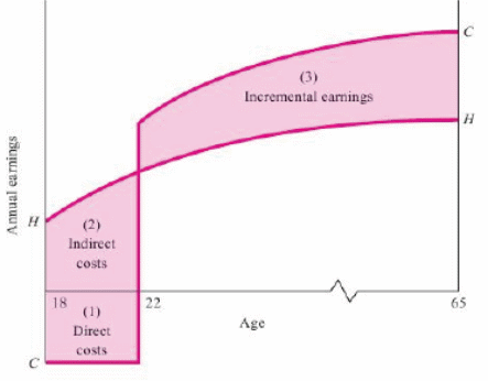
The first approach employs a discounting formula to compare the present value of benefits and costs. If an individual opts to join labor force market after completing high school education, his/her age-earnings profile will be HH. Conversely, if he/she opts to pursue college education, his/her profile will be CC (fig. 3). The internal rate of return (IRR) refers to the discounting rate in which the net present value of investment in human capita is equal to zero.
College wage premium is computed by comparing the percentage of college graduates’ earnings to those of high school graduates. Figure 4 show the wage premium for men and women between 1973 and 2008. According to figure 4, the wage premium ratios for men and women in 1973 were 1.38 and 1.48 respectively. In other words, college-educated men earned 38% (and women 48%) more compared to high-school graduates.
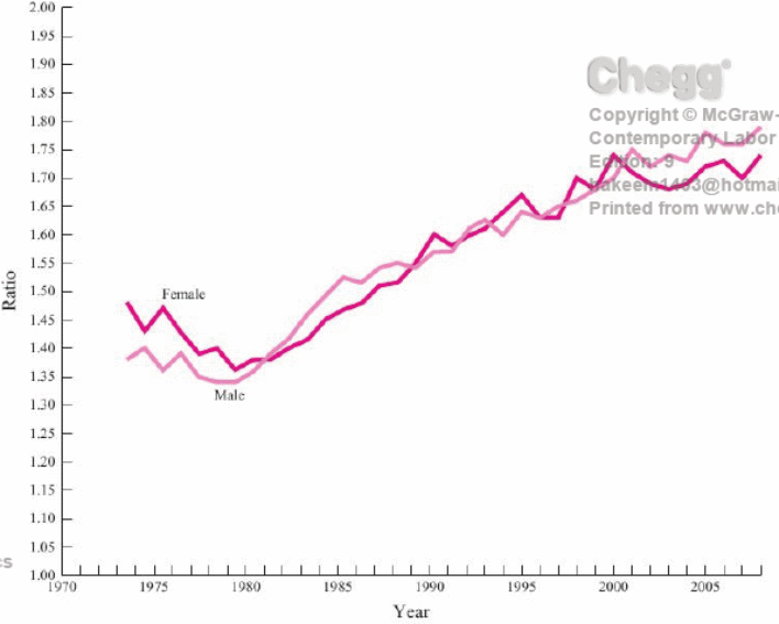
Figure 4 also shows that the wage premiums have risen considerably since 1979. It is worthy to note that the transformations in the demand and supply for high school and college graduates can be used to clarify the alterations in the wage premiums for college graduates.
Figure 5 shows both demand and supply curves which can be used to clarify why individuals invest different quantities of human capital to augment their earnings. There are three factors that can explain this phenomenon. They are: uneven access to credit facilities for human capital investment; variation in the ability to convert knowledge and skills into superior earnings; and variations in labor skills. Also, biases in the capital market usually underscore investment in real capital at the expense of human capital. The possible reason for these biases relate to the fact that human capital is personified in the borrower and thus it cannot be used as collateral.
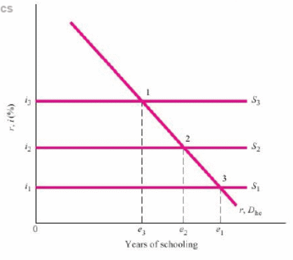
In addition, younger people are more likely to make investments in human capital than older people. However, younger people lack collateral assets or adequate credit ratings required to access loans for human capital investment. Thus, it is imperative that public subsidization is introduced to facilitate access to loans for human capital investment.
It is imperative that a distinction is made between general training and specific training. For example, general training enables an individual to gain skills that are applicable in all firms. On the other hand, specific training (also known as on-the-job training) enables an individual to gain specific skills that are only relevant for a particular firm. Since the labor force market is extremely competitive, some employees usually opt to pay for general training.
In addition, during the training period, these individuals often accept lower wages offered by the firm. There are several criticisms leveled against the human capital theory. For instance, the theory does not consider some education expenses as consumption. In addition, the theory ignores the fact that fringe benefits accruing from the jobs of college graduates are better than those of high school graduates.
The Demand for Labor
It is important to note that demand for labor is considered as derived demand. In other words, the demand for labor is subject to the goods/services its helps to create or provide. For instance, labor is demanded in the manufacturing sector because it plays an integral in the production of several products such as television sets and automobiles. Given that demand for labor is a derived demand, the power of the demand for any given form of labor is subject to the market value of goods/services created; and the contribution of labor in producing goods and services.
When all other factors are held constant, elasticity of demand for the labor curve (of a perfectly competitive trader) is higher compared to that of an imperfectly competitive trader. The explanation for this discrepancy is that the imperfectly competitive trader must decrease prices of his/her commodities in order to sell extra units of output.
Conversely, the perfectly competitive trader does not need to reduce his/her product prices. Figure 6 shows that the labor demand curve for a perfectly competitive trader slopes downwards due to diminishing marginal productivity. Also, figure 7 shows that the labor demand curve for imperfectly competitive trader slopes downward because marginal product reduces when extra units of labor are employed.
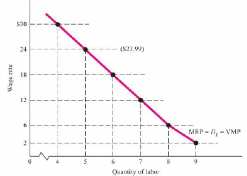
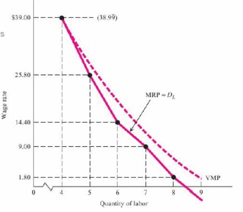
The elasticity of a long-term labor demand curve is higher compared to the short-term curve because a firm has adequate time (during long run) to alter non-labor inputs (i.e. capital). The market demand for a particular form of labor is less elastic compared to a plain horizontal summary of the short-run/long-run demand curves of individual firms. This is because firms hire more employees to increase output.
The wage elasticity coefficient (Ed) measures the changes in the quantity of labor demanded to changes in the wage rate. The coefficient of elasticity assumes a negative value because of the inverse correlation between the wage rate and the units of labor demanded. The demand for labor is elastic if Ed>1. On the other hand, If Ed<1, demand for labor becomes inelastic. The elasticity of demand for labor is subject to several factors such as: the elasticity of the product demanded; ratio of labor costs to total costs; the substitutability of other inputs (i.e. capital); and supply elasticity of other inputs. In addition, demand for labor is subject to various determinants.
These include: product demand (i.e. an increase in product demand will shift the labor demand curve to the right); the number of employers (i.e. demand for labor will increase when additional firms hire a certain type of labor); and the cost of other resources employed in production of goods and services. Therefore, the demand curve for labor will assume a new position when any of these three determinants of demand change.
During production, capital and labor are employed as either compliments or substitutes. For example, capital and labor are either gross compliments or gross substitutes if they are employed as substitutes in the production of goods/services. A change in the price of a resource (perceived as a substitute for labor) will change the demand for labor in either direction. If the resource is a gross substitute, the demand for labor will change in the same direction. However, if the resource is a gross complement, the demand for labor will assume the opposite direction. The theories of labor demand as well as elasticity of labor demanded have real-world applications. For example, these concepts are commonly employed in fast-food restaurants, textile and apparel industries.
Wage Determination and Allocation of Labor
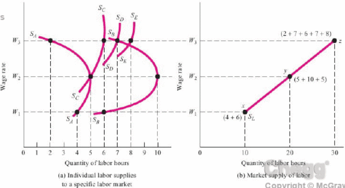
In a competitive market, an equilibrium wage and employment level can be determined using market demand and supply of labor. The positive correlation between wage rate and the amount of labor provided is depicted in figure 8. Figure 8a shows five distinct backward-bending labor supply curves for a certain market. On the other hand, figure 8b combines the supply curves to generate labor supply curve for the market. The opportunity cost associated with hiring the last worker (PL) is measured by the vertical height of the labor supply curve (xyz) of the market. Thus, the elasticity of labor supply curve diminishes as the time period reduces. In addition, when the wage rate rises in the short run, it may not bring about substantial increases in the units of workers in the market.
The labor market is likely to experience initial surpluses or deficits when the demand and supply of labor changes. Figure 9 shows that when labor demand reduces from D0 to D1 and labor supply rises from S0 to S1, there will be an excess labor supply (ab) at wage rate W0.
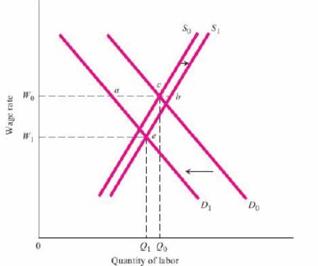
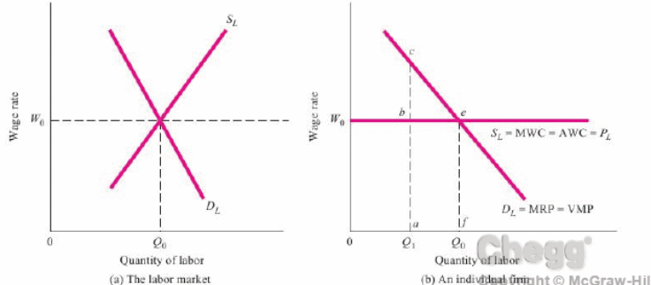
Accordingly, the wage rate declines to W1. Since the increase in labor supply is less than the decrease in labor demand, the equilibrium declines from Q0 to Q1. A firm that functions in an entirely competitive labor market is deemed as a wage taker. Figure 10a shows the labor market associated with a certain job-related group.
On the other hand, figure 10b depicts the demand and supply curves for a firm that employs this group. The firm’s decision to hire many workers cannot influence the market wage rate since the labor market is populated with other firms. Figure 10b shows that the firm lacks inducements to pay wages above the equilibrium market wage (W0). This is because the firm can employ as many workers as it wants at W0. However, if the wage offered by the firm is below W0, it will not attract any units of labor. Therefore, W0 (fig. 10b) is equal to the labor supply curve (SL) of the firm.
An efficient allocation of labor occurs when a firm acquires maximum amount of output from a particular quantity of labor accessible. In other words, an efficient allocation of labor occurs when the marginal productivity (MVP) of labor is equivalent to all other alternative employments. When a product market is dominated by a monopolistic firm, the marginal revenue (MR) declines faster compared to prices of products since additional workers are employed to increase output.
Given that product price (p) is less than MR, it follows that MRP will be less than VMP. When this happens, labor resources are underemployed and allocated inefficiently. When the labor market is characterized by monopsony, MWC will be less than PL since firms must increase their wage rates in order to attract more units of labor. As a result, the firm will hire fewer employees and pay them a wage rate that is less than MRP of labor. Thus, the aggregate value of output diminishes when labor resources are allocated inefficiently.