Introduction
Procedure
This report proposes a mathematical analysis of the ship towing problem. The speed and time data were collected during the tests and then processed using MS Excel. This included regression analysis as well as descriptive statistics. Most of the report calculations were done manually and the answers were checked on a calculator to maintain accuracy.
Results and Discussion
In this research report, four parts were conducted, each differentially evaluating the problem. Part A investigates the relationship between speed and time parameters for the ship during mathematical modeling. Part B uses the drag function to perform correlation and regression analyses to establish the effect of V on R/V. Part III focuses on estimating noise reliability in the context of SNR. Finally, Part D explores a case study that evaluates skills in using mathematical functions to find given values.
The nature of the relationship between speed and time variables
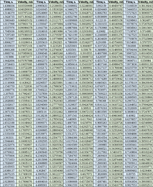
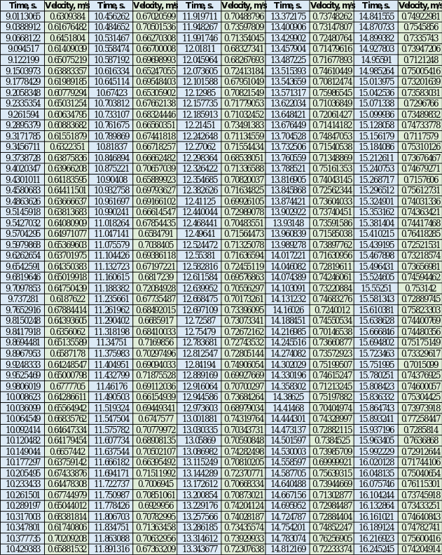
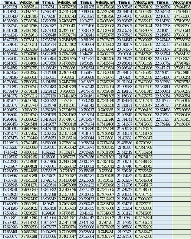
In the present part of the work, the interest was to find the nature of the relationship between speed and time variables to simulate the towing of a ship. A total of five trials were run, each of which automatically measured velocity values as a function of time: the first run was the most successful in terms of the data collected. Appendix A contains the raw data points, after cutting off the uninformative ends, for the first run; these values will be used throughout the report for analysis.
The primary task was to plot the data points on the scatter plot to form a general understanding of the structure of the relationship. Figure 1 provides information about this: generally, it is noticeable that the relationship between speed and time is non-linear, as initially, there is a mutual increase in the two variables, after which speed goes to a plateau, that is, it does not change its values significantly. It follows from this that when reaching some simulation conditions, the ship was practically in uniform motion, not changing its speed.
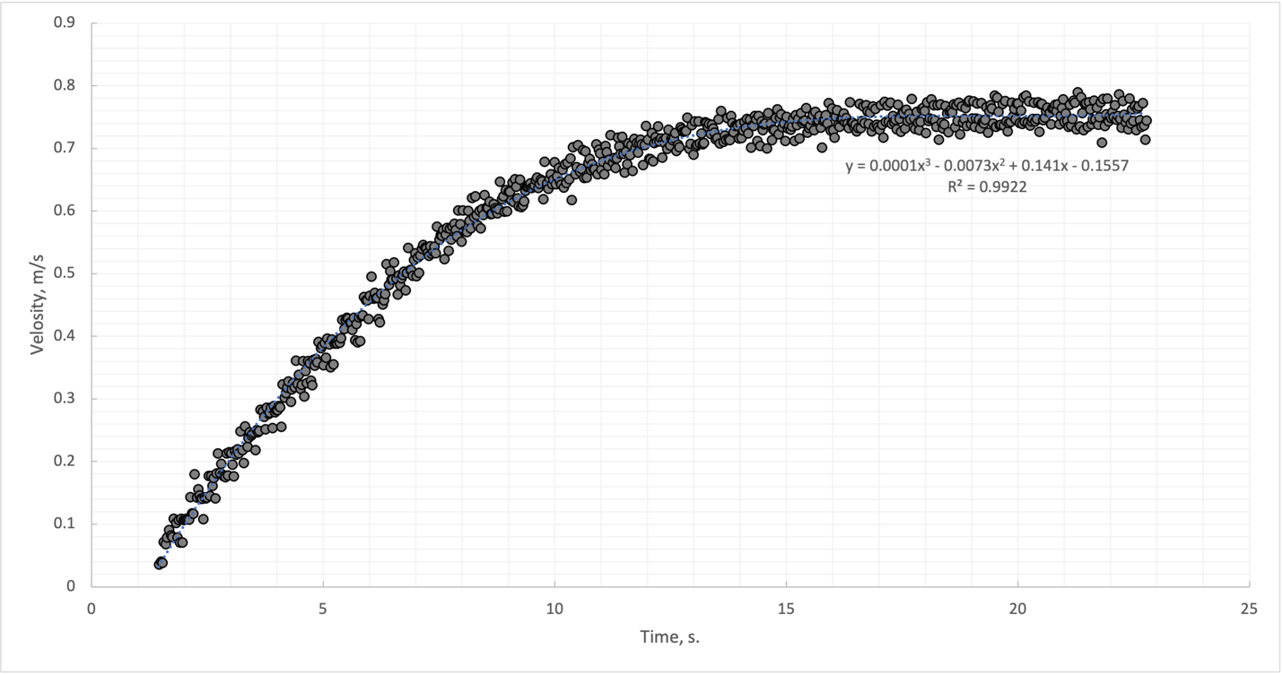
The dependence of velocity on time can be described in more detail using a trend line. As can be seen in Figure 1, this dependence is a polynomial function of the third degree, which allows us to obtain the best fit. The measure of this fit is the coefficient of determination, which determines the degree of variance coverage in the data (Chicco, Warrens, and Jurman, 2021). The higher this coefficient, the more accurately the regression line works. When the second-degree polynomial (parabola) was initially selected in MS Excel, the coefficient of determination was lower by about two percentage points, so increasing the degree by just one-unit increased reliability. At the same time, a further increase in the degree of the polynomial was inexpedient, as it made the rate function more complicated but did not significantly affect the coefficient of determination. Thus, the speed of this ship was determined by the following expression:
For positive values of time within the analysis, this polynomial was always greater than zero, from which it follows that the speed of the model ship was also always positive. This function can be differentiated to find an expression for the acceleration function. This is possible because the time derivative of the velocity determines the acceleration, that is, the change in velocity per unit of time. Thus, it is necessary to differentiate the third-degree polynomial by finding the parabolic acceleration function:

Just as the velocity function has been differentiated, it can also be integrable within a finite limit. Finding a definite integral characterizes the area under the original curve or, in physics terms, the work done (Strang and Herman, 2022). It is noteworthy that this area if found for a function of velocity versus time, determines the distance traveled by the ship model:

It follows from the above calculations that during the first approximately 21 seconds (exactly: 21.3211 seconds), the model ship covered a distance of 11.081 meters. If we count up from the start of the test, the total distance traveled is corrected to 11.996 meters. The intentional absence of rounding the time limits for integration was necessary to improve the accuracy of the calculations. It is noteworthy that the ship traveled approximately the same distance during all five launches. This is because the launches began at the same time and ended at the same time; if we accept the invariability of the external factors affecting the speed of the ship, the functions of this speed would have been approximately equal. With some assumption, the areas of the figures outlined by the velocity curves and horizontal axes in all launches were similar, with the only difference that statistical measurement errors can justify. Such errors could be due to systematic measurement errors, the influence of external factors such as air resistance, wind, and mechanical vibrations, and the choice of integration limits for each launch.
The regression analysis
Appendix B shows the data that was used to perform the regression analysis. Table 1 below shows the basic calculations that were used:
Table 1: Data needed for regression analysis
From this data, we can calculate the correlation coefficient r:
The obtained value indicates a high positive correlation between the data. The coefficient of determination can be obtained from r:
That is, the regression model can explain up to 95 percent of the variance in variable Y. The model itself has the following form:
where a can be calculated by the following formula:
And the coefficient b from the substitution of values for a particular point, for example (0.790, 0.241):
Then the final regression equation:
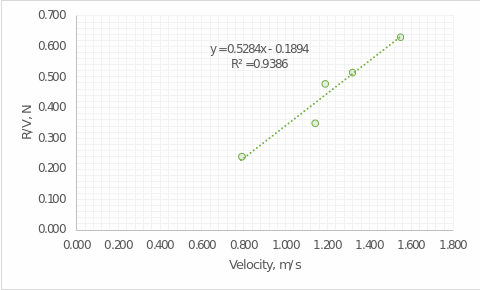
Interestingly, when V = 0, the function should go to zero since the resistance R should not exist at zero velocity, but the regression line shows a different value (-0.175). This is justified by the errors. In particular, a comparison of the calculated model with the proposed MS Excel calculations (Figure 2) shows close agreement between the two models. Any deviations could be justified by rounding during manual calculations.
Velocity
Some of the data shown in Appendix A and used for the analysis in Section 3.1 above turn out to be as close to the highest velocity value as possible. This occurs when the velocity function reaches a horizontal plateau and remains practically unchanged for the next seconds. For this region, shown in Figure 3, fifteen velocity and time values were isolated and entered into Table 2. These values will be used for the signal reliability analysis in this section of the paper.
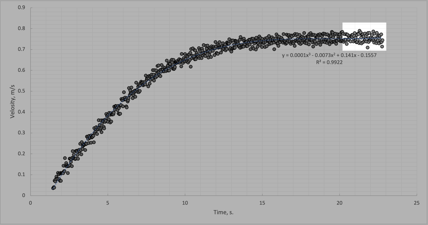
Table 2. Fifteen velocity and time values isolated from the maximum velocity region

For velocity sampling, it is possible to use descriptive statistics tools to calculate the mean and standard deviation. The sample standard deviation refers to the value by which, on average, each element in the sample deviates from the mean (Light, 2018). Then, the mean value for the rate in a given set is as follows:
And the standard deviation is:
Based on the two calculated results, it is possible to determine the signal-to-noise ratio (SNR):
In telecommunications, SNR refers to the ratio of the useful signal to any noise and interference that affects the quality of the signal transmission. For example, within the same apartment Wi-Fi signal can have different quality even in different corners of the room, which can be due to the influence of external noise on the signal itself. The quality of the transmitted signal under the influence of external factors is distorted, which affects the reliability of the received information and the load on the network (NetSpot, 2022). A great analogy for understanding SNR is a small room with many people in it, each talking to a partner, which creates background noise. Because of this noise, the information transmitted from one person to another can be distorted, cluttered, or disrupted, affecting the quality of communication. It is known that the higher the SNR value achieved for a particular signal transmission, the better the separation of useful information from interference and noise. There is a classification according to which the SNR with a value of up to 10 is considered extremely dirty, 10 to 15 inadequate quality, 15 to 25 moderate, suitable for everyday use of the Internet, and all values above are defined as high speed and signal purity (NetSpot, 2022). In the current calculation, the SNR turned out to be 39.461, indicating that this signal is critically clean and dependable; a huge amount of useful information compared to background noise is transmitted between receivers. Consequently, for signal transmission to achieve such SNR is extremely desirable.
The specific problem of modeling the towing of a ship
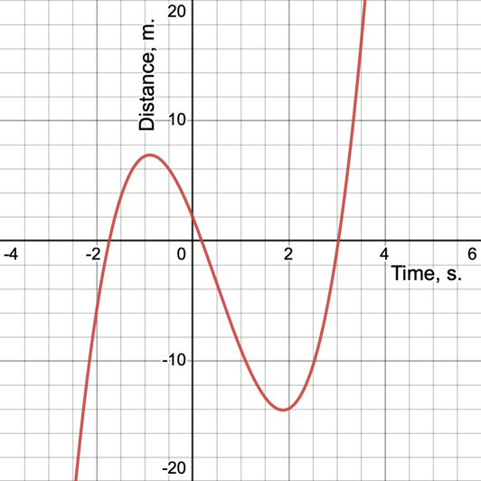
In this part of the research report, it is proposed to use the already learned mathematical skills to work with the specific problem of modeling the towing of a ship. In particular, it is assumed that the distance traveled function for the ship model as a function of time has the following form:
This is a cubic function, whose shape is shown in Fig. 4: as you can see, the path curve has a non-permanent trend, and is falling and rising depending on the selected time interval.
For this function, it is of most interest to obtain its derivatives, allowing a deeper evaluation of the dependence. In particular, the ratio of distance change to time change is the differential of this function and determines the velocity function, namely:
Accordingly, the velocity function is defined by a parabolic form and therefore shows both decreasing and increasing values. The value of the velocity at the end of the sixth second is determined from the expression:
Since the function is parabolic, with upward pointing branches, and has a y-intercept equal to (0, -10), the ship’s speed is zero at a certain point in time. This happens when the parabola crosses the abscissa axis, namely:
Solving the quadratic equation using the quadratic formula yields two roots that determine the moments of time at zero velocity:
Or rounded:
Both roots of the quadratic equation are the x-coordinates of the intersection of the parabola with the horizontal axis, which means that the speed at these times is zero. However, time cannot be negative, so the only appropriate value is 1.88 seconds. From the velocity expression, we can find the acceleration function:
And the value of the acceleration at the time t = 4:
The acceleration turns out to be zero at the next moment:
Finally, using the distance function, it is possible to find the total distance that the ship model traveled in ten seconds, namely:
Consequently, in ten seconds, the ship covered a distance of 1,602 meters.
Conclusion
This research report was devoted to mathematical modeling problems in order to study the experiment with towing a model ship. This report consistently examined aspects related to the nature of the relationship between speed and distance, regression analysis, and signal reliability. The manual calculations differed slightly from the automatic calculations by statistical parameters in MS Excel and were due to measurement errors and roundings as a result of the calculations.
Reference List
Chicco, D., Warrens, M.J. and Jurman, G. (2021) ‘The coefficient of determination R-squared is more informative than SMAPE, MAE, MAPE, MSE and RMSE in regression analysis evaluation’, PeerJ Computer Science, 7, pp. 1-24.
Light, G.L. (2018) ‘On the mean of sample-standard-deviation’, International Journal of Applied Mathematics, 31(3), pp. 359-370.
NetSpot (2022) What is signal-to-noise ratio and how to measure it. Web.
Strang, G., and Herman, E. J. (2022) Physical applications of integration. Web.
Appendix A
Initial Data Table
Appendix B
Source Data Table for Part B
