Introduction
When towing ships onto the water, it is critical to use mathematical modeling to minimize the risks of undesirable effects and to ensure increased accuracy of the process. This report uses speed, time, drag, and distance data from a variety of mathematical angles to determine aspects of such modeling. The work consists of four sequential parts in which velocity-time dependence is evaluated, correlation and regression analyses are performed, signal reliability is studied, and a practical example is given for given conditions.
Experimental Procedure
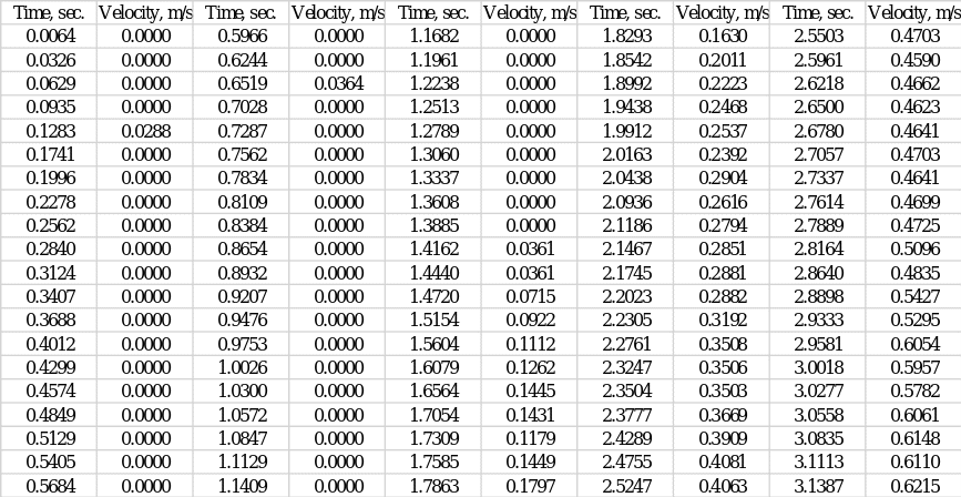
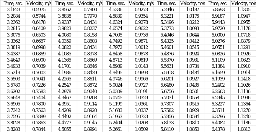
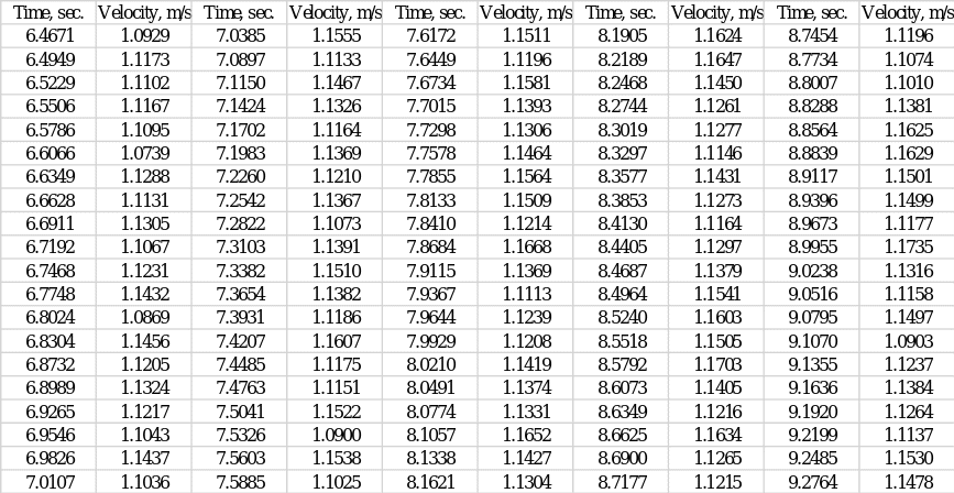
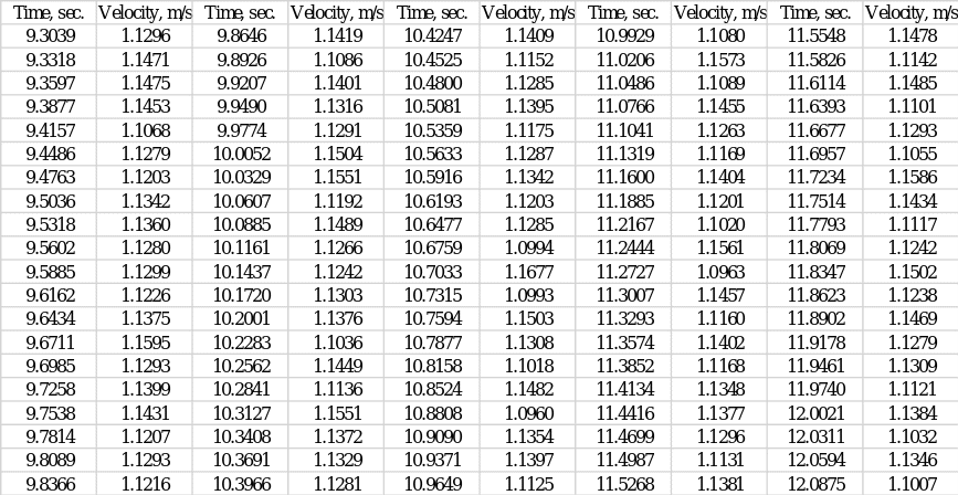
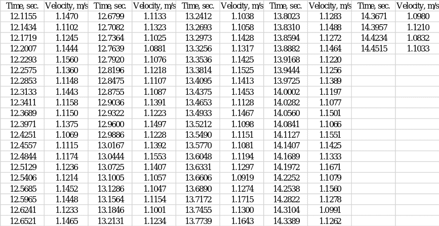
The towed model was fixed beneath the vehicle, with the end of the model aligned with the hydrofoils on the axis of the vehicle. During each of the runs, the velocity value of the model over time was recorded automatically; a total of five tests were performed. From them, the best-order data set (set #5) was visually selected, which was used in the report for the mathematical analysis. Calculations were performed manually, and visualizations were created using MS Excel.
Regression Model
Five repeated tests were performed to determine the relationship between speed and time for the ship model, among which the fifth showed the most acceptable and useful values for further analysis (Appendix A). Figure 1 below shows the graphical dependence of speed on time: one can clearly see that speed as a function of time initially has an upward trend and then goes to a certain plateau. Regression analysis was applied to the scatter plot, resulting in a best-fit curve. The coefficient of determination, R2, was used as a measure of this fit. This parameter indicates how closely the regression model is fitted to the data set; the numerical value of the coefficient of determination determines the level of variance of the data covered by the model (Turney, 2022). Figure 1 shows that the calculated R2 value for this model is.9905, which means that up to 99.05% of the variance of the data set is covered by the regression. This is an extremely high level, reflecting the excellent reliability of the model built.

It also follows from Fig. 1 that the regression equation, and consequently the velocity-time function, is polynomial and has the following form:
Analysis of this polynomial shows that in the case of zero time (t = 0) the ship would have a speed equal to -0.6611 m s-1. Obviously, such a value does not make physical sense, because it would mean that at rest the ship would have reversed direction of motion, which in reality was not observed. However, the non-zero velocity at zero time can be explained by the assumptions of the regression model, so the entire polynomial is recommended for analysis.
Differentiation
As it is known, the increment of velocity to the increment of time is a derivative function of the velocity that determines the acceleration of the ship. In terms of physics, this derivative shows the rate of change of the velocity function, that is, how much the speed of the ship changes over time, so the unit of this parameter is m s-1 by s-1 or m s-2. Consequently, it is possible to take the first derivative for the polynomial according to standard rules to find the acceleration function:
Notably, the acceleration function for the ship is expectedly parabolic, with the acceleration initially falling and then rising at the time interval of interest (approximately 0 to 15 seconds), as follows from Figure 2. A falling acceleration indicates a lower build-up of ship speed and vice versa. At the same time, this function never gives negative values for acceleration, which means that the ship’s speed never decreases, then if the object does not brake during the first fifteen seconds.

Integration
The velocity function for a ship can be not only differentiated but also integrated to find the antiderivative. In this case, the antiderivative of the original function will determine the path traveled by the ship in a particular time interval since the derivative of the path determines the speed. In terms of mathematical terms, finding the antiderivative for a velocity function determines the area bounded from below by the X-axis and from above by the velocity curve — the area of this figure (Figure 3) and determines the total path that the ship has traveled in the elapsed time (Gonzales et al., 2021). In order to integrate, it is necessary to use the period in which the original velocity function exists, namely from 0.0064 seconds to 14.4515 seconds; rounding, in this case, would prove unnecessary, as it would compromise the accuracy of the result. Accordingly, to find the integral from the velocity function, it is necessary to solve the following:
The solution of this integral is also performed according to standard rules, namely:
As expected, the degree of the polynomial grows when searching for the antiderivative. Then the obtained function defines the path function for the ship as a function of time:
If the original time limits of the integration are substituted, it becomes possible to determine the total distance traveled by the ship during this time, namely:

From the calculations shown above, it follows that in 14.4451 seconds the ship covered a distance of 12.71 meters.

It is worth noting that if each of the five tests began at the same time and ended simultaneously, then within the statistical error due to some discrepancy in the data between tests, each of the ships in the five launches traveled the same distance equal to 12.71 meters. The significance of this equality of areas under the velocity curve is built on the assumptions of equality of velocities in all tests and the slight error in the data.
Correlation Analysis
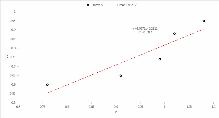
V and R/V values were determined for the resistance curve obtained during the measurement: the results are shown in Table 1. In addition to information on the measured data, Table 1 also contains information on the calculation of the coefficients required for the regression analysis.
Table 1: Table of initial resistance curve data and coefficient calculations for further use

The data obtained above will be used to calculate the Pearson correlation coefficient. It is worth specifying that the numerical value of this coefficient determines the direction and strength of the relationship between two quantitative variables. For the current case, the coefficient is equal to:
r=n
Consequently, for a set of variables the coefficient of 0.914. This implies that there is a positive, strong relationship between them, which means that an increase in one of them leads to an increase in the other.
Regression Analysis
For the data given in Table 1, it can also be calculated the slope coefficient of the regression line:
slope=a=n
The obtained value of the slope in the regression line confirms the conclusions of the correlation analysis and shows a positive relationship between the variables. It follows that an increase in V for every one unit leads to an increase in R/V by 1.109 units. However, it is also necessary to determine the value of RV when V turns out to be zero, i.e., the y-intercept:
y=ax+b
y=1.109x+b
For the specific point (0.76, 0.60):
0.60=1.109(0.76)+b
0.60-1.109(0.76)=b
0.60-0.84284=b
b=-0.24284
This indicates that when V is zero, the R/V function has a negative value. Then, the general regression equation:
y=1.109x-0.243
The resulting calculations can easily be checked using the built-in analysis in MS Excel. Figure 4 shows a graph of the dependence of R/V on V and also describes aspects of the regression analysis. As can be seen from the equation shown in Figure 4, it is almost identical to the manually calculated one, but there are some discrepancies. These deviations are caused both by rounding used in the manual calculations and by not selecting a specific point to calculate the y-intercept.
The Region Near Maximum Ship Speed
For the fifth data set, fifteen points were selected in the region near maximum ship speed, for which velocity and time values were measured. Table 2 contains information about these points.
Table 2:Data on 15 points of velocity and time measured near the area of maximum ship speed
MS Excel was used to calculate the mean and standard deviation values for these data; the results are shown in Table 3.
Table 3:Results of calculation of descriptive statistics for velocity
On the basis of these data, it becomes possible to determine the signal-to-noise ratio (SNR) for the ship. It is worth noting that SNR is an indicator determining the power of the useful signal in relation to the background noise. Background noise can include any interference that affects the quality of the signal as it travels, which includes mechanical, electromagnetic, thermal, and other factors. In analog and digital devices, SNR is used as a measure of the reliability and accuracy of received data, as higher values of the coefficient respond to better signal transmission (Chen et al., 2019). In telecommunications technology, low SNR is undesirable because it makes it more difficult to isolate useful, information-carrying signals from background interference. In turn, low SNR becomes the cause of the necessity to repeat data transmissions, which creates additional load on the network and increases the waiting time. The calculated SNR value for fifteen points is as follows:
As it is known, an SNR above 20 usually defines a good signal that can be used for signal transmission (Baker, 2020). However, for the current dataset, an SNR of about twice that value was obtained. This indicates excellent results, which means that this signal can be used for telecommunications because it is good at distinguishing the useful signal from the background noise.
Case Study of Ship Motion
This part of the paper investigates a case study of ship motion for which a time-dependent path function has been specified. As stated earlier, the derivative of the path is velocity, so for a given function, it is possible to determine an expression for velocity according to standard rules, viz.:
The velocity function turns out to be parabolic, with upward branches, which means that the velocity of the ship increases over time. At time t = 6, the value of the ship’s velocity is equal to:
It follows that after six seconds, the speed of the ship is equal to 170 m s-1. The velocity function can be analyzed in a different way, namely in order to find the time value when the velocity turned out to be equal to zero. In terms of graphical representation, this will be the x-intercept of the point at which the y-value (speed) turns out to be zero:
As expected, the quadratic equation gives two roots, but one of them is negative. Time in the context of the physical sense cannot be negative, so the only appropriate answer is a time value of 1.88 seconds. It is at this point in time that the ship’s velocity function turns out to be zero — the object is not moving.
The velocity function can also be differentiated to find the acceleration function, which is equivalent to the second derivative of the path:
The acceleration function has a linear ascending form, from which it follows that the acceleration of the ship was constantly increasing. At time t = 4, the acceleration can be found as follows:
That is, the acceleration after four seconds of motion was 42 m s-2. If the acceleration was zero, that is, the object was moving at a constant speed, this was achieved at the following point in time:
Finally, for the original path function, one can find the total distance the ship traveled in the first ten seconds, which is:
Conclusion
This report investigated mathematical modeling for ship towing. The report included areas of analysis such as correlation, regression, descriptive statistics, differentiation, and integration. The results include the following conclusions:
- The relationship between speed and time for the model was not linear.
- The dependence of R/V on V was defined as a linear upward trend with a strong positive correlation.
- The SNR for the data was determined to be robust.
Reference List
Baker, A. (2020) what is SNR and how does it affect your signal? Web.
Chen, Y., et al. (2019) ‘Improving the signal‐to‐noise ratio of seismological datasets by unsupervised machine learning’, Seismological Research Letters, 90(4), pp. 1552-1564.
Gonzales, K. et al. (2021) 4.2 Determining area under a curve. Web.
Turney, S. (2022) Coefficient of determination (R²) | calculation & interpretation. Web.
Raw speed and time data for the fifth set (Part A, Part C)