Monopolistic competitive market is a market structure in which firms have many competitors, but each firm sells slightly differentiated products.
Monopolistic competitive firms cannot earn economic profit in the end because in the short run they earn supernormal profit. This attracts new firms into the market in the long run given that the monopolistic market barriers to entry are low, firms have good knowledge of the market and there is an opportunity for the new firms to start up with their own way in differentiating their product to appear unique from their competitors.
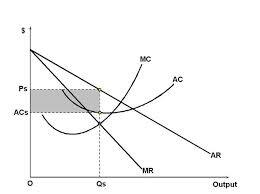
Monopolistic competitive firms in the short run earn supernormal profits as indicated below.

As new firms appear in the market, the demand for the existing firm products tends to be more elastic and the demand curve moves to the left, decreasing the set prices. Eventually, the supernormal profit is eliminated.
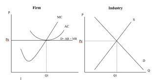
Monopolistic competitive firms in the end
As supernormal profit attracts new firms into the market, the demand curve of the existing firms shifts to the left. This means that firms have managed attain their long run equilibrium.

In a monopolistic market, the prices are higher and the quantities are lower because they determine the prices being aware of the fact that the consumer has no other alternative.
A relatively inelastic demand curve favors the producers because a huge change in price results to an insignificant change in the quantity. Consumers have to bear with changes in prices because there is no alternative available in most cases. In an elastic demand curve, a slight change in price causes a great change in the quantity demanded. This is illustrated in the diagram above.
Homogenous products of a duopoly market
Firm 1’s profit maximizing quantity
We know that average revenue is (AR) =P (price), this means that P=300 – 3Q=AR
Therefore, to get total revenue (TR), we will have to multiply AR by Q (quantity). TR= Q*AR= 300Q-3Q^2
At a maximum profit, marginal revenue (MR) = marginal cost (MC)
We have to differentiate TR in order to find MR, thus after differentiating TR we find our MR to be 300-6Q. Using the rule MR= MC, we equate our values of MR and MC
300-6Q=100, after solving for Q we find the value of Q=33 1/3
But we know that Q=q1+ q2 therefore, 33 1/3= 50+ q2 we have to solve for q2= -16 2/3 when q1=50
When q2=20, we use the equation to find the value of q1,
33 1/3= 20+q1 and after simplifying the equation the value of q1 is 13 1/3
Pa= 11+ 9/20Pb, Pb=11+9/20 Pb,
For easy computation, let’s assume that Pa=p1 and Pb=p2 therefore,
No variable costs
p1= p1q1 = p1(90-2p1+p2) =90p1 – 2p12 + p2p1
dp1/dp1=90-4p1+p2 =0 or
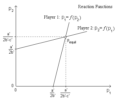
p1=(90+p2)/4 (Reaction function of firm 1)
Similarly, p2=(90+p1)/4 (Reaction function of firm 2) Comparison between Bertrand and Cournot Competition:
Example: q1=90-2p1+p2, q2=90-2p2+p1
Bertrand Competition: p1*=p2*=30, q1*=q2*=60, p1 = p2 = 1800
