Introduction
The least squares method should be used for deriving the best fit line based on observed data of certain variables. The outcome of this method is to reduce the sum of squares of errors which can be found in an equation (Björck, 1996). This method applies to the regression analysis. In this paper, regression analysis is performed to predict the relationship between the time series (independent variable) and the time spent watching television each day measured in minutes (dependent variable).
Regression #1: Original Data
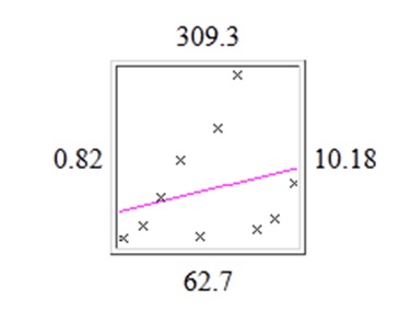
First set of data which has 10 observations has been used for carrying out the regression analysis using the model.
The graph presented below shows the best fit line for the data selected over 10 observations. The vertical distance between the actual values and best fit line which is drawn upon the predicted values can also be observed from this graph. The graph indicates a positive correlation between two variables selected for the regression analysis as the slope of the best fit line is positive.

This is further supported by the predicted values obtained from the regression analysis. It could be indicated that the predicted values are increasing over the time series. On the basis of this assessment, it could also be indicated that there is not a perfect linear relationship between time series and duration of time in minutes spent by individuals watching television.
Table #1: Predicted Values of y.
Regression Equation
The regression equation derived from the analysis is provided in the following:
y = 6.37576 x + 105.533
Where y = Predicted mean value of dependent variable i.e. time in minutes spent watching television
x = Value of independent variable i.e. time series
The regression equation indicates the y-intercept, B0 has a value of 105.533 whereas the coefficient of slope, B1 has a value of 6.37576. This affirms the positive relationship between time series and the amount of minutes spent watching television. The mean value of the dependent variable is predicted to increase over the period of time. The higher the x value the higher it can be estimated that the value of y will be.
Regression Coefficient
From the regression analysis the regression coefficient has been obtained as r = 0.257174 which implies that the regression model has been able to predict only 25.72% of the total variations observed in the dataset and the remaining 74.28% is residual as determined by the sum of square. The ability of the regression model could therefore be considered as weak and on the basis of this it could be suggested that the dataset must be extended to include additional number of observations or the model must include other variables which could have implications for the human behavior of watching the television on a day to day basis.
Regression #2: Extended Data
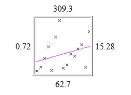
The second dataset that has been used for performing the regression analysis comprises of additional observations over an extended time series. It is expected on the basis of the results of the previously performed regression that by increasing the number of observations in a dataset the ability of the regression model to predict the relationship between the dependent and independent variables is likely to improve. Using the same regression model available the following graph has been obtained which indicates the best fit line. From analysis the graph it could be suggested that by increasing the number of observation the difference between the predicted values and actual values included in the dataset has improved. The best fit line overlapping the actual values has improved by increasing the number of observations. The relationship between two variables included in the regression analysis that the number of minutes spent watching television and time series still appears as positive which implies that the time spent into front of television increases over a period of time.

The table provided below indicates the predicted values using least square method. Also from the table an outlier could be indicated at observation number 7.
Regression Equation
The regression equation derived from the second regression analysis performed is given as:
y = 4.825 x + 111.133
From this equation, it can be indicated that the coefficient of intercept, B0 is 111.133 and the coefficient of slope, B1 has a value of 4.825. The value of coefficient of slope has reduced as the number of observations is increased. The relationship between times and the amount of time spent watching television remains positive which implies that the mean value of the dependent variable increases over the period of time.
Regression Coefficient
The regression coefficient that has been obtained from performing the regression analysis is r = 0.311247 which implies that the revised regression model is able to predict 31.12% of the total variations observed in 15 entries into the dataset. This suggests that the regression model is still able to predict small proportion of the total variations observed in the dataset and there are still 68.88% of variations still unexplained by the regression model. The regression coefficient has improved from 0.257174 to 0.311247 by adding to the number of observations. This implies that the ability of regression can be improved if the size of the dataset is increased. Smaller samples tend to have more variations and therefore undermine the ability of the regression analysis and the results presented from a study.
Conclusions
Regression model is a model to predict the relationship between two or more variables. It helps in predicting how the value of one variable changes with changes in the mean values of other variables (Kedem & Fokianos, 2002). For this paper, there are two regression models implemented to predict the relationship between time series and the amount of time measured in minutes watching television and it is clear that there is a positive relationship between both variables. Moreover, the statistical testing of data suggests that by increasing the number of observations to be included in a sample for testing can improve the ability of the regression model to determine the relationship between variables.
Reference List
Björck, A. (1996). Numerical Methods for Least Squares Problems. Amsterdam: SIAM.
Kedem, B., & Fokianos, K. (2002). Regression Models for Time Series Analysis. New York: John Wiley & Sons.