Statistics: Data and Business Decision-Making Report

Executive summary

This is a data analysis of SHV Pty LTD customers who patronized the business in the year 2011. The customers have been selected randomly for this analysis. This paper aims to find out the type of customers who patronize the business in terms of gross annual income, gender, marital status, family status, employment status, and distance from the store. These factors have been analyzed to come up with a conclusion, which may help the company to grow.

Introduction

Every store needs to know their target market to stock the right product as well as offer the right discounts to the customers. This information is obtained by analyzing the existing customers of the company. At the first, instant one may see that there are so many products offered in the market but a close look will reveal that it is not true. Not all these products are targeted to the same population. Instead, they have their niche market. These product features are different and obviously, the price the customer prepared to pay is also more or less depends on the product features or positioning. Different customers see the product differently and their assessment of the product is different. The same cup of coffee in a fast food shop or ordinary shop may cost less when compared to the price it is charged in a five-star hotel. The service is different in both cases(Freytag and Clarke, 2001).

Market Segmentation can base on variables such as geographic, demographic, and psychographic. The purposes of customers using patronizing are looking for price, proximity to destination, product quality, etc. The expectation of the customer varies depending upon the variables discussed above.

Data analysis

Gender

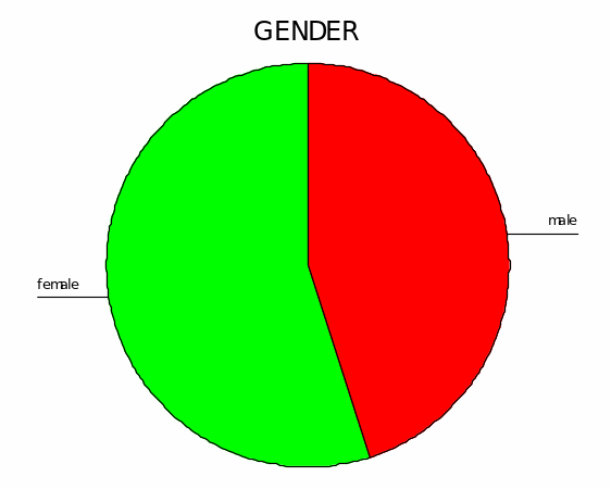
The sampled population had 36 males and 44 females. This frequency is represented in the table and the graph below.

Gross income and average spending

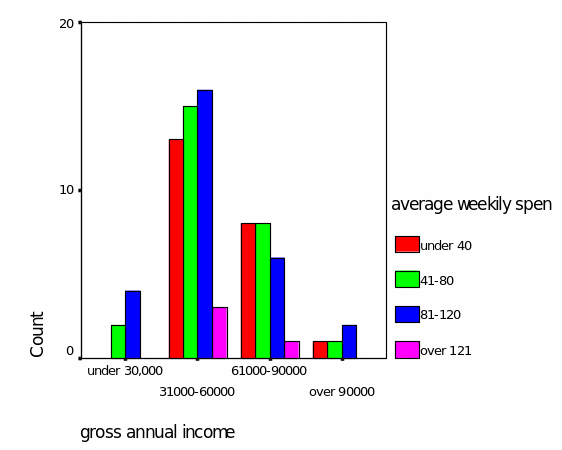
From the table below we can state that those people who spend less than 40 were 22 and non of them had an income of under 30,000 most of them had 31,000 -60,000 while over 90 there was one person. Those people who spent between 40 and 80 were 26 as most of them were from the category of the annual income of 31,000to 60,000. However, in this category, some people were earning fewer than 30, 000 who made purchases. Among those people who spent over 80-, 120 included four earning less than 30,000, 16 earning between 31,000 and 60,000.

Gross annual income * average weekly spending at stores Cross tabulation

Count

Level of education and weekly spending

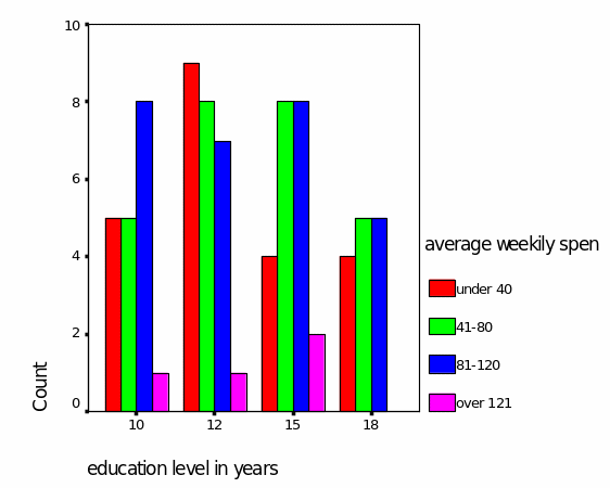
Among the customers sampled 19 of them had 10 years level of education 25 had 12 years, 22 had spent 15 years to acquire education while 14 had completed 18 years of education. Among this 22 had spent less than $ 40 and they were 5 with 10 years of education, 9 with 12 years, 4 had 15 and 18 years of education each. For those who had spent $81 -120, 8 had 10 years of education, 7 had 12 years, 8 with 15 years and 5 had 18 years of education.

Education level in years * average weekly spending at stores Cross tabulation

Count

Marital status * average weekly spending at stores Cross tabulation

Count

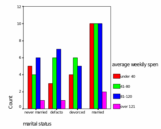
From the table above averagely the married people spent a lot, followed by the defacto, then the never married and finally the divorced. Whereby the majority spent $81-120 as only four spent over 121. This is a clear indication that the married spent a lot due to increased household size or increased number of a dependant.

The household size and the expenditure

Number of people living at home * average weekly spending at stores Cross tabulation

Count

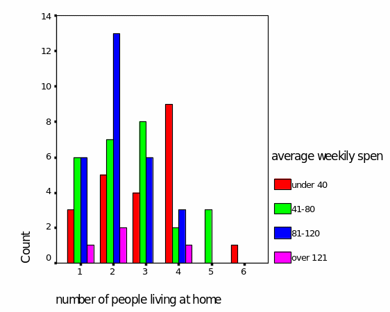
The house with a small household that is one and two family members spent the most amount as compared to other household sizes, whereby their expenditure was ranging between 41- 80 averagely to most of them. Very few of them spent over $121 weekly.

The relationship between the selection of products and weekly expenditure

Average weekly spending at stores * store has a good selection for product Cross tabulation

Count

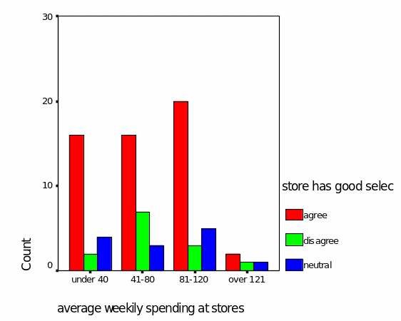
Most people agreed that there was a good selection of products thus, they spent a lot as a few were disagreeing that the selection was not good.

The link between the store operating hours and expenditure

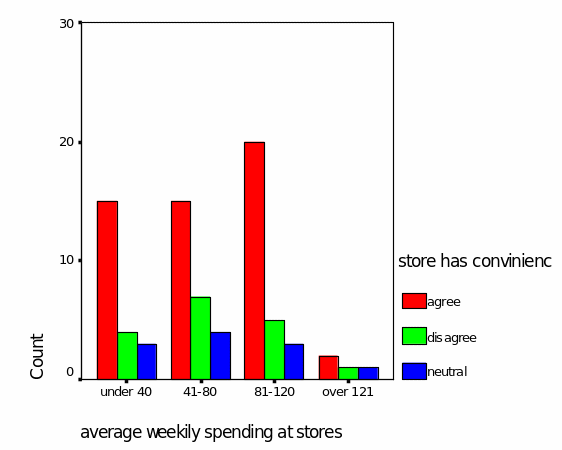
The expenditure was good as indicated by most of the customers who admitted that the store’s operating hours were very much convenient to many of them. Very few people were not favored by the store’s operation time (Gore and Altman, 1992).

Average weekly spending at stores * store has convenience operating hours Cross tabulation

Count

Inferential statistical technique

We want to test whether the average spending of the customers is equal regardless of the distance between home and the store. The hypothesis for the study will be:

• H_O : μ₁ =μ₂ =μ ₃
• H_1: at least one mean is different(Creswell, 2005)

Reject the null hypothesis if t-calculated is greater than t-critical.

Paired Samples Correlations

The relationship between the distance covered to the store and the amount spent is not strong because it correlates 0.033. at 0 there is no relationship and at one there is a strong positive relationship while at negative one there is a strong negative relationship.

Paired Samples Test

From the output above t-calculated are 2.328 at 95% confidence level and t –critical is1.96. since t-calculated is greater than t- critical, we reject the null hypothesis and therefore conclude that there is sufficient sample evidence at 5% to suggest that the average weekly spending at the store is different for various customers covering different distances between home and the store.

Regression

The question is whether there is a difference between the means of spending for males and females, in this case, the alternative and null hypothesis will be:

• H_O: μ₁ -μ₂ =0
• H_a : μ₁ -μ₂ ≠0 (Aron, Aron and Coups, 2006)

The following is the output from SPSS at a 5% level of significance. Using the statistics shown below we accept the null hypothesis if the p-value is less than 0.05. gender only affects the weekly spending by 1.5% as the rest is contributed by the income level, the number of household size, the marital status, the distance between the store and home and finally the sore’s selection for goods.

Model Summary

Predictors: (Constant), GENDER

Anovs

• Predictors: (Constant), GENDER
• Dependent Variable: average weekly spending at stores

Given the above p-value of 0.284 and an F-test of 1.163, we conclude that average spending in the supermarket is not influenced by the gender of the customer.

Chi-test

To carry out the chi test for this store the following questions have to be answered.

• Q1: is there evidence to reject the claim that the advertised merchandise was in store?
• Q2; is there evidence to accept the hypothesis that the store has convenient operating hours?
• Q3: Is there proof to reject the claim that the store has a good selection of products?
• Q4: is there evidence to accept the hypothesis that the store has the most competitive pricing in this suburb?
• Q5: is there evidence to reject the claim that the distance between home and the store affects the weekly spending?

Test Statistics

To answer the above questions the following are the hypothesis for each question:

• Q1; H_O: the advertised merchandise was not always in store
• H_a: the advertised merchandise was always in store
• Q2; H_O: the store has no convenient operating hours.
• H_a: the store has convenient operating hours.
• Q3; H_O: the store has no good selection of products.
• H_a: the store has a good selection of product
• Q4; H_O: the store has no competitive pricing in this suburb
• H_a: the store is the most competitive in this suburb
• Q5; H_O: the distance between home and the store affects the weekly expenditure
• H_a: the distance between home and the store

The next step is to find the critical chi- values at a 5% level of significance. The following are the critical values for the teaching question.

• Q1: the degrees of freedom are 5-1 =4 giving a critical value of 9.488.
• Q2; the degrees of freedom is 3-1=2 giving a critical value of 5.991
• Q3; the degrees of freedom is 3-1=2 giving a critical value of 5.991
• Q4; the degrees of freedom is 2-1=1 giving a critical value of 3.841
• Q5; the degrees of freedom is 4-1=3 giving a critical value of 7.815

In question one we reject the null hypothesis because the critical value is less than the calculated value, therefore we conclude that the advertised merchandise was always in store.

In question two we reject the null hypothesis since the calculated value is greater than the critical value therefore, we can summarize that there is enough evidence to suggest that the store has a convenient operating time.

Also in question three we reject the null hypothesis and accept the claim that the store has a good selection of products. In the question we too since the calculated value is less than the critical value, we accept the null hypothesis that the store has no competitive pricing in the suburb. Finally, in question five we reject the null hypothesis and accept the claim that the distance between the home and the store influenced the customers.

Discussion

Annual income appeared to be influencing weekly purchases by an individual at the store. Most people who had income ranging between 31,000 -60,0000 appeared to be the largest shoppers followed those earned between 60,000-90,000, those who earned less than 30,000 are not a good target market for the store, although the few who turned up for shopping spent between 40,000 and 120,000 per week. Another category that the market was segmented was the level of education and most people who had the education of 12 years and 15 years preferred the store. It was noted also that those who had 10 and 18 years levels of education patronized the sore in large numbers though the majority of them spent less than $ 80 per week, while the other levels of education covered between $40-120 per week.

Marital status was found to be another factor that affected spending at the store. Customers who are married were found to be good spenders in the store and those who never married were very few but they also spent between $40-120 per week. It appears that the amount spent by an individual was not influenced by the marital status, but the marital status influenced his or her patronizing the store. This observation is made from the fact that the largest number of people was married.

The store appears to attract customers who came from households with two people. The majority of the people who spent more than $81 were from this category, while those who spent between $40 -80 were from a household of their people. It is interesting to note that those households with more than five people are not a target market for the store because only four customers were sampled from this category.

The products available for selection in the store influenced the customers in spending his money because the majority of the people agreed that a good product influenced the spending. There is a linkage between the store-operating hour and customer expenditure. Most customers viewed the store as having a convenient operating time, which favored most of the customers(Griffith and Pol, 1994). While shopping it is easy to find the product of our choice and it provides the customer the convenience of shopping while at the store. Convenience is an important thing for most customers as most respondents had a strong feeling that it was convenient. The analysis done from the t-test shows that the average spending of customers at the store was different for customers coming from different distances between home and the store. However, it was noted that there was no strong relationship between home and the store and the amount spent. There was also no relationship between the gender of the customer and the amount he spent in the market(Hooley and Saunders, 1993).

Chi-test analysis shows that the store had the merchandise they always advertise as well as those items were competitively priced. An effective marketing communication strategy should make a business thrive amidst fierce competition. From the initial step of raising products’ awareness to segmented marketing, marketing communication strategies should be infused with innovation, integrated communication plans, and strong public relationship measures(Green, 1979)

Conclusion And Recommendation

The analysis has shown that many factors influenced a customer who patronized the store. Most customers were enticed by a selection of products available, the convenience of operating time the pricing offered by the store, and their levels of income. Pricing and promotion are very important to any marketer who wants to understand the market he is operating in. this store will help to upgrade its competitive position within the market as well as increase the market shares. The dividing of the market into groups with similar characteristics such as gender, levels of education, annual income, marital status. Household size, employment status, and the years that have lived in the suburb will help to design a good marketing strategy that will reach the target customers. The information will also be useful in the decision-making of the management on expansion strategy(Bowonder, Dambal, Kumar, and Shirodkar, 2010).

Besides the predictions for the future being good for retail marketing, the current business scenario for the store also looks impressive. The retail marketing environment seems to be resilient, which is proof of the convenience that it affords. But the fact that online sales will increase substantially this year demonstrates the resilience of the channel and is a testament to the value and convenience most customers find when shopping. Companies strive to improve the shopping experience of customers, as there is a lot of competition in the field.

Reference List

Aron, A., Aron, E., & Coups, E. J. 2006. Statistics for psychology. Pearson: Pearson Prentice Hall.

Bowonder, B., Dambal, A., Kumar, S., & Shirodkar, A. 2010. Innovation strategies for creating competitive advantage. Research Technology Management, 53 (3), p. 19-32.

Creswell, J., 2005. Educational Research: Planning, Conducting, and Evaluating Quantitative and Qualitative Research. New Jersey: Prentice-Hall, Inc.

Freytag, P. V., and Clarke, A. H 2001. Business to business segmentation, Industrial Marketing Management, 31, 4, pp.475–86.

Gore, S., & Altman, D.G., 1992. Statistics in Practice. London: British Medical Association. New York: Wiley,

Green, P. E 1979, A new approach to market segmentation, Business Horizons, February, pp.61–73.

Griffith, R. L., & Pol, L. A 1994, Segmenting industrial market, Industrial Marketing Management, 24, pp.38–46.

Hooley, G. J., and Saunders, J. A 1993, Competitive Positioning: The Key to Market Success, Prentice Hall.