Study of Natural Circulation in a System With a Rectangular Contour Essay

Introduction and Background information

Natural circulation flow system is a simple phenomenon occurring in fluids courtesy of density and temperature gradients in a force field. Basically, this system constitutes a heat sink and a heater, with the former positioned higher than the later, and “both coming in contact with a portion of the fluid” (Lehmann 78). In a synopsis, whatever happens is that a section of the fluid becomes heated by the virtue of heat fluxes, becomes less dense and rises. On the other hand, the cooled section becomes dense and hence drops by gravity. As such, these fluid motions results in a circulation.

The advantage of a natural circulation system is that it requires minimal maintenance costs since it doesn’t use forced convectional equipments like pumps and fans. Moreover, it is advantageous in systems that employ natural circulation “as primary heat transfer mechanism in order to optimize the thermal performances and avoid unwanted dynamic behaviors, such as flow instabilities and flow reversals” (Lehmann 79).

Natural circulation loops (NCL) find applications in a wide scope of engineering aspect including geothermal processes, nuclear power generation, solar heaters, cooling small electronic like devices e.g. computer processor exacter. To enhance the performance of NCL to suit the various engineering aspects several models were developed and researched. Initially designed models (heat points) were found inefficient owing to flow reversals. To curb this recent models have been developed including toroidal and rectangular RCL. However, the later is less stable.

In a nutshell, the aim of this experiment is to use the NCL (rectangular loop) to draw a correlation between the flow rate and the system temperature and hence, compare it with the theoretical relation shown below:

Description of Experimental Setup

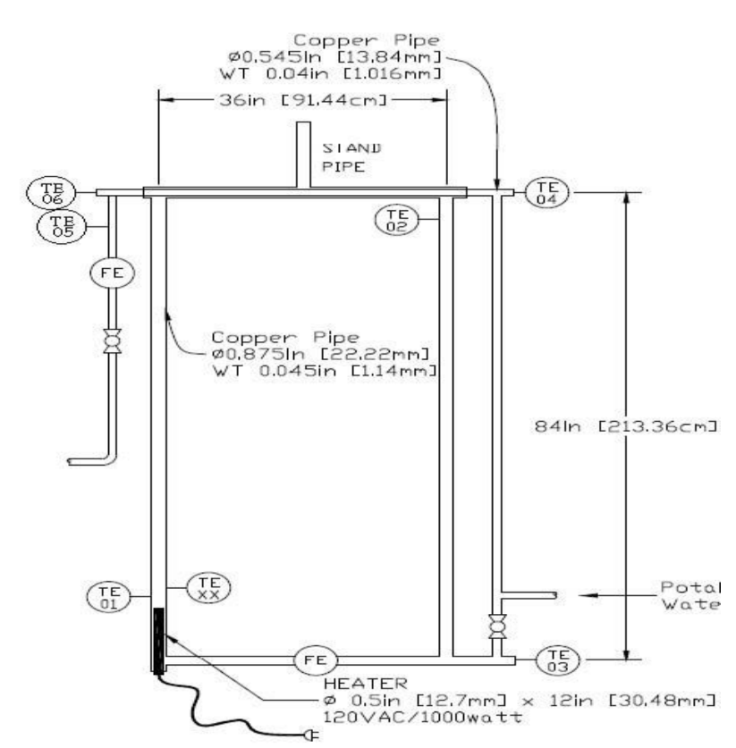
The experimental setup consists of a rectangular loop (Figure 1) constructed from copper tubing, and a data acquisition and display system with an inbuilt storage abilities. The parameters present in the data are obtained from two flow meters and four thermocouples designated as below on the loop diagram:

• TE01-hot leg temperature near heater outlet (C°);
• TE02-cold leg temperature near cooler outlet (C°);
• TE03-cold leg temperature near cooler inlet (C°);
• TE04-cooling water temperature near cooler inlet (C°);
• TE05-cooling water temperature downstream of cooler outlet (C°);
• TE06-cooling water temperature near cooler outlet (C°);
• FCM801-cooling water flow rate (Kg/hr);
• FCM802-primary water flow rate (Kg/hr).

List of Equipment

• A simple natural circulation loop.
• Agilent 34970A Data Acquisition Switch Unit (DASU).
• RS-232 data cable.
• Agilent BenchLink Data Logger Software.
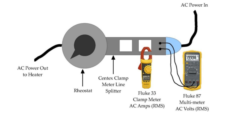
• Centex Clamp Meter Line.
• Fluke 330 Series Clamp Meter.
• Fluke 87 Digital Multi-Meter.

Procedure

The procedure for this experiment was divided into three categories. These categories were data acquisition setup, system setup, and data processing. With regards to data acquisition setup, the series clamp meter, digital multi-meter and the DASU systems had to undergo energizing prior to running of the Agilent Benchlink Data Logger Software. With the aid of a screen the desired time was set, and all parameters vital for the experiment confirmed. This was followed by system configuration and hence ready for data acquisition.

With respect to system setup, the water in the expansion tube was adjusted to approximately half the tube before running the system. The cooling water flow (FCM801) was run at 7.5±1 Kg/hr with the rheostat set at ‘10’. With the rheostat set at ‘25’ and, at a steady state, the values for voltage, current and time stamp were recorded. The same procedure was run with the rheostat set at ‘50’ and ’75.’ Similarly, with FMC801 operating at 15±1 kg/hr, the same procedure was run with the rheostat set at ’25,’ ’50’ and ’75.’ The rest of the data was collected from the data file. The data file had to undergo modification before analyzing using MATLAB.

Data

Table 1: parameters measured at steady state.

Table 2: operating points, flow rates and the difference between Q_in and Q_out.

Analysis

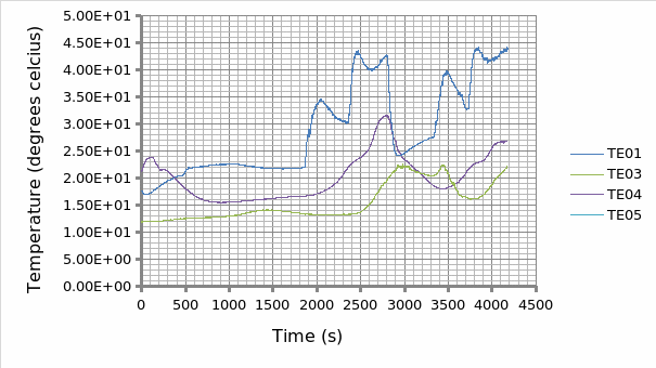
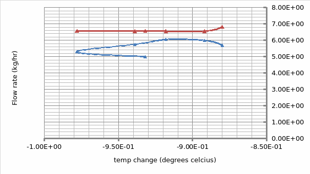
The time range where the six operating points were approximately steady is between 20.05.6 and 21.02.6 seconds.

The average of the below parameters measured over the steady state time range are:

• 101: 17.800°C
• 900: -0.329°C
• 901: -2.120°C
• 903: 11.100°C
• 904: 99.800°C

For the six operating points, the equation below will aid in finding the heat transferred into the primary water (Q_in) and, into the cooling water (Q_out).

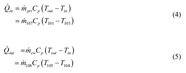
For instance, for the first operating point:

• Q_in = 5 * 4.18 (17.5 – 12) = 121.62 kJ
• Q_out = 6.57 * 4.18 (23.8 – 12) = 324 kJ

The rest of the operation points are shown in table 2 above.

Discussion

The objective of this experiment was to investigate a natural circulation in a rectangular loop system and hence draw a correlation between the flow rate and the temperature. From the experiment as displayed by the above graphs (1 and 2) the trend agrees with the theoretical however; the results were not accurate. To this end, this has a bearing on the experimental design which gave room for the discrepancies. For instance, the timing could have been poor because of the manual control systems. To eliminate this then the future experiments ought to be automated.

Works Cited

Lehmann, Walter. Atomic and Molecular Structure: the development of our concepts, San Francisco: W.H. Freeman & Co., 1972. Print.