Demand is the quantity of products customers are willing to buy at a particular price while supply is the quantity of products firms are willing to offer for sell. There is an inverse relationship between demand and supply when all other factors remain constant. On the other hand, market equilibrium is attained at the point of contact between the equilibrium quantity on offer and the equilibrium price in the market. Here, the market is defined as buyers and sellers. The demand and supply for a product influence each other.
When equilibrium is attained, no changes in price occur. However, if the price of the product falls below the equilibrium price, the demand for the product is in excess creating a shortage. Here, shortage occurs when the quantity in supply is lower than the in demand. At this point, sellers provide fewer products than the quantity consumers are willing to buy.
When the price of a product is increased, positive changes in supply and demand occurs. Raising prices decreases excess demand for a product and cancels out the demand and supply differences, restoring the supply and demand equilibrium.
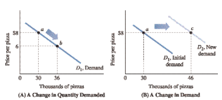
If supply exceeds demand, and the price reaches above the equilibrium point, the price is reduced by excess supply and causes the demand for the product to reduce. In this case, the gap between the quantity in demand and the quantity supplied reduces. An equilibrium point is attained when the demand and supply are the same. As exemplified in figure 1 below, when changes in quantity of the product in demand changes, there are changes in the supply of the product, shown in the movement of the arrow between points a and b.

Figure 1
There is a change in the quantity in demand as the line shifts from a to b and a change in demand as the graph in B above shifts toward the right direction. There is also a change in the product prices when the variables that cause changes in demand are factored into the graph shown above.
Factors such as increase in income, increase in the price of substitute goods, decrease in income, and changes in complementary factors cause changes in the curve. Complimentary factors include inferior, normal, preference, and substitute goods. A shift to the right influences the demand, supply, and product pricing positively.
The change is caused by increase in population, decrease in the prices of complimentary goods, expectation of higher future prices, and changes in consumer preferences. Therefore, a decrease in demand decreases the equilibrium price as mentioned above. A decrease in equilibrium price is caused by excess supply underpinned by decrease in the price of substitute goods, decrease in income, population decrease, and price increases of complimentary goods.
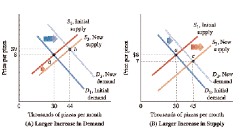
The changes in supply and demand have simultaneous effects on the market equilibrium. As illustrated in figure 2 below, the market equilibrium shifts to point b from point a, because demand exceeds supply. Here, a large increase in demand causes a sharp increase in prices. On the other hand, quantity increases with an increase in demand and supply.

Figure 2
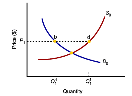
Market equilibrium is attained when the quantity in demand equals the quantity being supplied as shown in figure 3 below. At this point, prices do not increase.

Figure 3
Contact point