Introduction
Engineering calculations in the aviation industry are required to include measurements of the strength of the parts used, as this information is fundamental to improving flight safety. This paper uses data on the time it takes for parts to fail in 36 measurements. The general idea behind the measurements is that failure rates for parts tend to change over time, and the use of a Weibull distribution density function is aimed at studying these dynamics. The Weibull function is commonly referred to as an exponential density distribution that shows the dependence of failure rates on time (de Jonge, 2021). The mean and standard deviation through variance calculated for the density distribution allow the central trends for the failure rate to be determined. These values are subsequently used to determine the confidence interval and interpret it in the context of the company evaluating the parts for failure.
Calculations and Answers to Questions
Primary to the calculation of the Weibull distribution is the definition of the Beta parameter, a shape parameter that describes the behavior of the failure rate. In other words, based on the value of this coefficient, it is possible to determine the dynamics of order frequency (CFI Team, 2022). MATLAB software and program code written by Omid Alavi were used to calculate the Beta coefficient using current data on the time it takes for a part to fail (Alavi, 2014). The calculated beta value was 1.63; the distribution then takes the form as shown in [1].

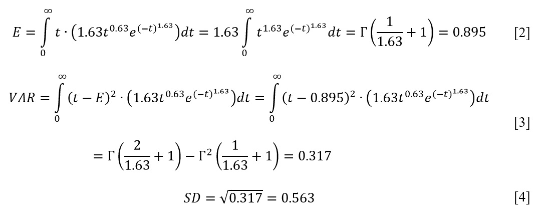
To calculate the expected value (E) and variance (VAR), the corresponding values of the integrals were determined, as shown in [2] and [3]. The integrals were calculated automatically using the free Wolfram software calculator. Thus, the expected value for this distribution was determined to be 0.895, which in turn was used to calculate a variance of 0.317 (Ahmed, 2015). In this case, the standard deviation is the square root of the variance and equals 0.563, as shown in equation [4].

Based on the information obtained from these calculations, it can be seen that the average value for this probability density function is 0.895, from which it follows that the part with a high probability will be damaged under load before the end of its service life. In addition, from the calculated value of the beta parameter (>1), it becomes clear that the failure rate tends to increase over time, which corresponds to the reduced wear resistance of the material, as confirmed by the histogram in Figure 1 (Weibull, 2020). In other words, there is a high risk that a part will fail during use, as empirical data shows. Consequently, customers need to be made aware of these risks.

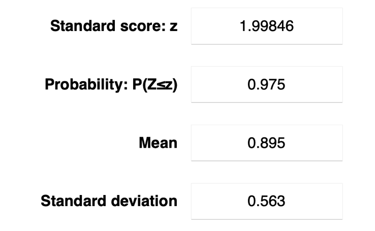
The critical value allows defining a threshold against which one can be determine whether a part is vulnerable in terms of extrapolation to the general population and make a decision based on this data. To calculate the critical value, it is assumed that a given distribution meets the conditions of normality, so it is acceptable to use the Normal Distribution Calculator from Stat Trek (Stat Trek, 2020). Previously obtained values were used for the calculation, as shown in Figure 2. The automatic calculation shows that the critical level z is 1.998.

For the calculated critical value, it is also possible to calculate the lower and upper bounds of the confidence interval using the formulas [5] and [6]. As can be seen, the 95% confidence interval for this mean value was 95% CI [0.864, 0.926]. This means that there is a five percent probability that the true mean for the general population is not in this interval. For a company that tests products for durability and reliability, using these bounds would allow determining the expected failure rate: values above the confidence interval would signal increased failures and the need to urgently revise production standards, while lower values, in contrast, would allow judging production optimization. If the failure occurs within that confidence interval, however, the company need not worry because the sample mean does not necessarily indicate the truth of the population mean; that is what the acceptable lower and upper bounds are used for.

Conclusion
This paper used the Weibull distribution to estimate trends associated with part failure rates in the aviation domain. The test information contained information about the time after which the part was partially or completely failed under load. The best fit value of the shape parameter (1.63) was chosen for the Weibull distribution, and the mean (0.895), variance (0.317), and standard deviation (0.563) were calculated. A 95% CI [0.864, 0.926] confidence interval was constructed at 95% significance. The boundaries of this confidence interval contain information about the population mean – in other words, the true value of the mean time to failure is between 0.864 and 0.926. This information, combined with the calculated value of the shape parameter (β>1), indicates a trend of increasing failure rates over time, which the manufacturing company should pay attention to.
References
Alavi, O. (2014). How can we calculate Weibull Scale and Shape parameters using Moment method (given in attachment)? ResearchGate.
Ahmed, A. (2015). Mean and variance of the weibull distribution. StackExchange.
Stat Trek. (2020). Normal distribution calculator. Stat Trek.
Weibull. (2020). Characteristics of the Weibull distribution. Weibull.
de Jonge, B. (2021). Weibull distribution; Weibull parameter estimation. YouTube.
CFI Team. (2022). WEIBULL.DIST function. CFI.