Wal-Mart Employee Satisfaction Survey Essay

Introduction

Wal-Mart is a leader in the retail industry. However past research revealed that this retail giant remunerates its employees at rates that are on the lower side. A recent survey drawn on a sample of 100 interviews was conducted to determine employee job satisfaction. The findings show that Wal-Mart employees are not happy with their pay check.

Findings

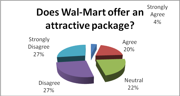
As the pie chart below shows, 54% of the employees surveyed feel that the ‘salary and benefit package’ that Wal-Mart gives them is not attractive.

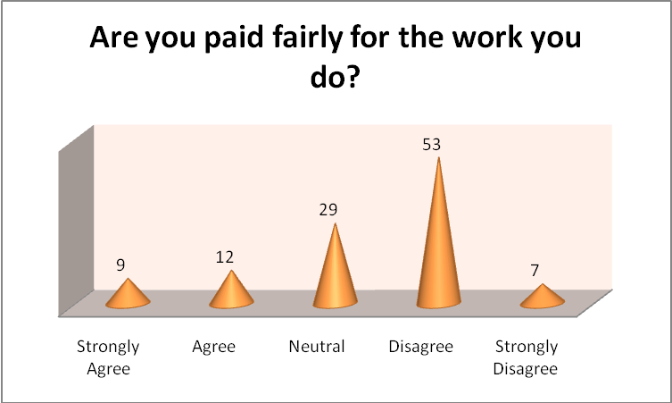
This concurs with the general feeling 60% of the employees have that the pay they receive is not commensurate with the work they do as shown in the corn bar graph above.

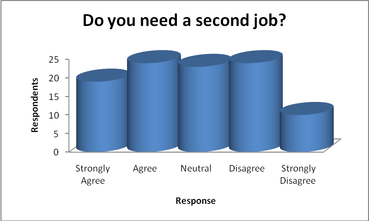
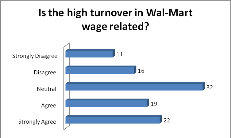
As the visual below (right) shows, most of the respondents (19% and 24%) were in need of a second job. A good number (24%) do not need a second job. When asked whether the high turnover in Wal-Mart had any connection with wage rate many (32%) were

Noncommittal although a good number (19% +22%) felt that there was a connection (see bar graph above, on the left). For more details see the summary table in appendix 1.

Hypothesis testing

A hypothesis is an “assumption [made] about a population parameter” (Levin and Rubin 1991 p.346). The objective of this exercise is to test the population mean of Wal-Mart employees.

Hypothesis statement

The null hypothesis (H₀) is that the ‘population mean’ (μ) is equal to the hypothesized mean (μ_H0) which is 550 stated as: H_0: μ = μ_H0=550. The alternative hypothesis (H_a) is that the ‘population mean’ is not 550. This creates two alternatives: μ is less than 550 or μ is greater than 550. This is statistically stated as: H_a: μ ≠ μ_H0, which gives raise to: H_a: μ < μ_H0, or H_a: μ > μ_H0.

Significance level

A 5% level of significance has been predetermined for this test. This means that the probability of committing a type I error is 0.05.

Test statistic

The preferred test statistic for this test is ‘z’ because it is the best method for “comparing the mean of a sample to a hypothesized mean for a population”(Kothari 2003 p.237).

Decision rule

A confidence level of 5% means that the acceptance region will take 95% or 0.95 of the normal distribution curve area. Being a two tailed test, there will be two critical values (“the values that lie exactly on the boundary of the region of rejection” (Zikmund p.502).).Half of 0.95 is 0.4750 which reads a ‘z’ of 1.96 in the normal curve area table. With δ_p given as 33 and n as 100 the critical value for the lower region is μ-zδ_p÷ SQRT of ‘n’ or 550-(1.96x(33÷SQRT100)) which gives 543.5. Critical value for the upper limit is 556.5. The decision rule is to reject H_0, if the ‘sample mean’ (X bar) appears outside the critical limits.

Sample and decision

From a sample of 100 employees interviewed; the mean score (X bar) on the five point scale on the survey question ‘Do you feel like you are paid fairly for the work you perform?’; equaled 20 (see appendix 2). The sample mean is outside the critical region on the lower side or H_a: μ < μ_H0 because 20<550. Therefore the decision is that the population mean is no longer 550 and hence the null hypothesis should be rejected.

Appendix 1

Summary Table Wal-Mart job satisfaction survey

Appendix 2

Sample mean (X bar) for the survey question ‘Do you feel like you are paid fairly for the work you perform?’

References

Kothari, C.R., (2003). Research Methodology: Methods & Technique, 2^nd Edition. India. Wishwa Prakashan.

Levin, R.I. & Rubin, D.S. (1991), Statistics for Management, 5^th Edition. USA. Prentice-Hall International Inc.

Zikmund, W.G., (2008). Business Research Methods, 7th Edition, USA. South Western