Introduction
The purpose of the present report is to determine if there is a direct correlation between the age of drivers and blood ethanol concentration after a car crash. In order to achieve the desired goal, a set of data consisting of eight variables was used. The variables included gender of the driver (categorical), age of the driver (continuous), type of car crash (categorical), the blood level of tetrahydrocannabinol in ng/ml (continuous), blood ethanol concertation (ml/L), cannabis preparation (categorical), and neuromuscular coordination score (continuous). The sample size was 363 participants, among which 141 were female, and 222 were male. The present report uses descriptive statistics, an independent sample t-test, and Pearson’s R to perform the analysis.
Background Information
Drinking and driving is responsible for a car percentage of car accidents worldwide. According to Zhao, Zhang, and Rong (2014), alcohol consumption contributes between 31% and 34% of traffic accidents in different countries of the world. Empiric research demonstrates that ethanol concentration in the blood of drivers affects their concentration, attitude, judgment, vigilance, perception, reaction, and controlling (Edvardsen et al., 2017; Zhao, Zhang, and Rong, 2014).
In particular, higher ethanol concentration in the blood of drivers is associated with impulsive and adventurous behavior, and the speed of driving is positively correlated with the amount of alcohol consumed (Zhao, Zhang, and Rong, 2014). Even though recent research demonstrates that mono-intoxication rarely becomes a cause of fatal accidents, alcohol consumption is associated with an increased chance of administering illicit drugs, which positively influences the chance of fatal accidents (Edvardsen et al., 2017). Since drinking leads to dangerous behaviors on the roads, higher ethanol concentration is associated with higher chances of fatal traffic accidents.
Different age groups administer alcohol with different patterns. In particular, the age group between 18 and 24 consumes the highest amount of alcohol; however, the 25-44 age group consumes almost as much (CDC, 2017). From 45, the average alcohol consumption steadily decreases with an increase in age (CDC, 2017). However, alcohol affects different age groups with different intensities. Older people have a lower tolerance to alcohol, as muscle mass is replaced by fat tissue as people age (DrinkWise, no date). This implies that older people will have a higher ethanol concentration in their blood than younger people.
At the same time, the bodies of older people experience more difficulties with excretion of alcohol (DrinkWise, no date). Moreover, due to polypharmacy, there is a high risk that alcohol will cause adverse drug events, which may lead to impaired driving (Edvardsen et al., 2017). Thus, alcohol has different effects on the body, depending on age.
In general, younger people drive less responsibly than their older counterparts do (Sivak and Schoettle, 2011). This implies that even small doses of alcohol taken by younger people can lead to fatal accidents (CDC, 1983). Therefore, it is crucial unclear if there is a correlation between the age and the drivers and the ethanol concentration in their blood after car accidents. The present report aims at closing the identified gap in the literature.
Data Analysis
Descriptive Statistics
Descriptive statistics is crucial for data analysis, as it helps to visualize the raw data provided in a dataset. Descriptive statistics include the measures of central tendency and dispersion. The measures of central tendency include mean, median, and mode, while dispersion can be measured by variance, standard deviation, minimum, maximum, range, etc. The most important descriptive statistics are mean and standard deviation (SD). Table 1 below demonstrates descriptive statistics for the two variables analyzed in the present paper.
Table 1. Descriptive statistics.
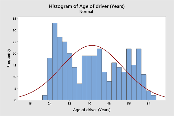
According to the information provided in Table 1, the age of sampled drivers ranges between 21 and 66, with a median age of 40. The mean age of drivers (41.05) is close to the median value, which implies that the distribution is not skewed. SD of the drivers’ age is 12.35. Thus, according to the central tendency theorem, 68% of all the drivers in traffic accidents are between 28.7 and 53.4, while 95% of drivers are between 16.35 and 65.75 years of age (Curtis and Drennan, 2013). Figure 1 below demonstrates visualizes the data using a histogram with a fitted normal distribution curve.
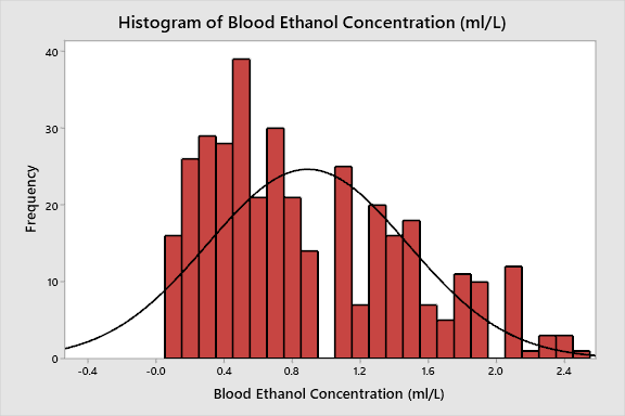
The blood ethanol concentration of participants varies between 0.1 ml/L and 2.5 ml/L with a median value of 0.7. Since the mean value (0.89) is higher than the median value, the standard distribution curve will be right-skewed. SD of the parameter is 0.59, which implies that 68% of drivers will have ethanol concentration between 0.3 and 1.48 (Curtis and Drennan, 2013). The data is visualized in Figure 2 below.
Parametric vs. Non-Parametric
Parametric statistics are used to make inferences about population parameters based on a sample (Curtis and Drennan, 2013). Both variables analyzed in the present paper can be used for parametric tests, as they adhere to the basic assumptions. The first assumption of the parametric tests is normality, which implies that the data is normally distributed along the x-axis. Figure 2 demonstrates that Blood Ethanol Concentration is normally distributed, as the histogram follows the normal distribution curve with the right skew. Even though the age of drivers does not exactly follow the normal distribution curve, the data is symmetrically distributed from both sides of the mean values, which is considered acceptable to assume normality.
Another assumption that should be made for parametric tests is independence. This implies that all the samples taken should be independent of each other. This assumption can be made from the dataset characteristics, as there are no signs of the samples being dependent. Finally, the parametric correlation test (Pearson’s R) assumes a linear relationship between the two variables. Since the description of data does say otherwise, this assumption can be made. In summary, since there are no indicators of the non-parametric nature of the data, a parametric test will be conducted to make inferences.
Differences in Means
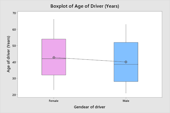
Before conducting the correlation analysis, it is crucial to understand if the mean age of drivers and the concentration of ethanol differ depending on the gender of the driver. Two independent t-tests were run to understand if there was a statistical difference between mean values in the two continuous sets of data selected, as split by gender. The first test revealed that the difference between the mean age of female drivers (M = 42.8, SD = 11.8) and the mean age of male drivers (M = 40, 12.6) was statistically significant at alpha = 0.05 (t(313) = 2.13, p = 0.034). The null hypothesis was that there was no significant difference in the mean age of males and females that experienced car accidents, while the alternative hypothesis was the there was a significant difference. In statistical terms:
Where:
μ1- mean age of female drivers
μ2- mean age of male drivers
The null hypothesis was rejected since the p-value was below the identified alpha for the test. It should be noted, however, that a lower significance level (for example, alpha = 0.01) would have affected the conclusion. The test results are visualized in Figure 3 below.
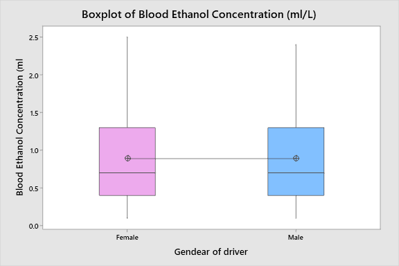
The second test revealed that that the difference between the mean blood concertation of ethanol in females (M = 0.889, SD = 0.628) and mean blood concentration of ethanol in males (M = 0.89, SD = 0.562) was statistically insignificant at alpha = 0.05 (t(313) = -0.01, p = 0.991). The null hypothesis was that there was no significant difference in the mean blood ethanol concentration of males and females that experienced car accidents, while the alternative hypothesis was the there was a significant difference. In statistical terms:
Where:
μ1- mean blood ethanol concentration of female drivers
μ2- mean blood ethanol concentration of male drivers
The conclusion was made since the p-value was above the identified alpha for the test. It should be noted that any reasonable significance level would not affect the results of the analysis, as the p-value was very high. The results of the second t-test are presented in Figure 4 below.
Correlation
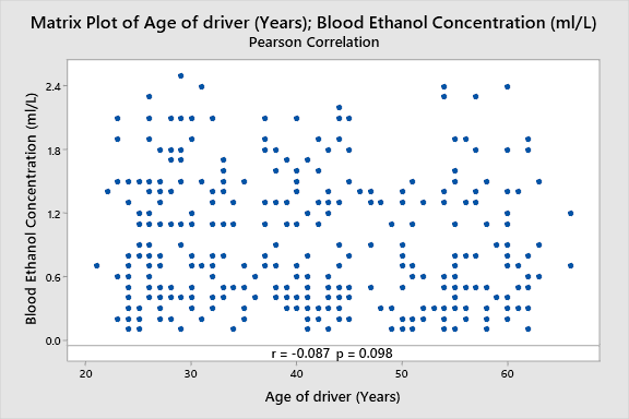
There several basic tests that can be used to calculate correlation between two variables. Pearson’s correlation coefficient (Pearson’s R) is the most commonly used parametric test to assess correlation. The results of Pearson’s R analysis produce a ratio between -1 and 1, where -1 is the strongest negative correlation, 1 is the strongest positive correlation, and 0 is an absolute absence of correlation between two variables. The analysis of the correlation between the age of drivers and blood ethanol concentration revealed a very weak negative correlation (r = -0.09, p = 0.1).
Moreover, the correlation coefficient may be statistically insignificant if the selected alpha is below 0.1. Thus, it may be concluded that there is no significant correlations between the age of drivers and blood ethanol concentration. This can be seen in Figure 5 below, as there is no evident pattern of relationship between the two variables.
Conclusions
The analysis of statistical data led to several conclusions. The primary purpose of the present report was to understand if there was a correlation between the age of drivers and blood ethanol concentration. The results revealed no significant correlation between the two matters. This implies that the average blood ethanol concertation does not differ considerably depending on the age of drivers, which is consistent with the literature review provided in the present report. According to the CDC (2017), the amount of alcohol consumed decreases steadily after the age of 45. This is confirmed by Pearson’s R, which was found to be negative. However, according to DrinkWise (no date), the decrease in consumption of alcohol can be offset by a decrease in alcohol tolerance and excretion. This fact explains the high p-value and the low correlation coefficient of Pearson’s R analysis.
Another conclusion that can be drawn from the analysis presented in the present report is that blood ethanol concentration does not depend upon the gender of the driver. In other words, the mean blood ethanol concentration of females does not differ significantly from the mean blood ethanol concentration of males. According to the CDC (2017), the consumption of alcohol differs between males and females. In general, women consume less alcohol than males (CDC, 2017). However, this fact does not influence the mean blood ethanol concentration in drivers.
Another crucial conclusion that can be made is that the average age of females who experienced car accidents is higher than the average age of males. This is consistent with the trends in the composition of drivers. In particular, according to Sivak and Schoettle (2011), the mean age of female drivers is high on average than the mean age of males. This is associated with the fact that women receive their driver’s licenses at an older age. Thus, the results of the analysis are consistent with the existing literature.
When considering the results of the analysis, it is crucial to acknowledge the limitation. First, the analysis is made based on a limited amount of data. Even though the sample size is adequate for making inferences, it is unclear if the sampling methodology was adequate for parametrical tests to be applicable. Second, the results of the analysis are applicable only to drivers who experienced car accidents. This implies that it would be inappropriate to translate these results to other populations. Finally, the explanations of the results are based on the reviewed literature. However, there may be other explanations to these facts.
Reference List
CDC (1983) Blood alcohol concentrations among young drivers. Web.
CDC (2017) Alcohol consumption. Web.
Curtis, E. and Drennan J. (2013) Quantitative health research: Issues and methods. Open University Press.
DrinkWise (no date) Age and alcohol: understand the effects of drinking as you get older. Web.
Edvardsen, H. E. et al. (2017) ‘Differences in combinations and concentrations of drugs of abuse in fatal intoxication and driving under the influence cases’, Forensic Science international, 281, pp. 127-133.
Sivak, M. and Schoettle, B. (2011) ‘Recent changes in the age composition of US drivers: Implications for the extent, safety, and environmental consequences of personal transportation’, Traffic Injury Prevention, 12(6), pp. 588-592.
Zhao, X., Zhang, X., and Rong, J. (2014). ‘Study of the effects of alcohol on drivers and driving performance on straight road’, Mathematical Problems in Engineering, 2014, article 607652.