Introduction
SAAM II, which means simulation, analysis, and modeling software II, is pharmacokinetic analysis software designed for studies of radioactive experiments. The software is very popular among biomedical and bioengineering experts. As such, the package is a very dominant instrument in research, education, and project development (Burnham 12). The system provides help for biomedical problems and services through consultation on the use of software analysis and kinetic data. With the help of the software, an individual can design multi-compartmental representations, simulate experiments on these representations, and analyze data using the designed representations. There are two ways of creating these models. These are by means of compartmental and numerical applications.
Designing the models using compartmental and numerical application methods
This enables the user to come up with visual symbols of the models graphically. The model can be illustrated with the help of differential equations. Algebraic equations are generated with the help of numerical applications. For both methods used in designing SAAM II models, simulation of complex experimental designs can be achieved. After designing the models, the user can solve the samples before fitting them to the data with the help of special mathematical and statistical methods.
With the help of the SAAM II compartmental application and a set of model building tools, an individual can illustrate compartments and represent transfers and delays on a drawing board when required creating graphical symbols of the required compartmental models. Thereafter, the user is required to describe the attributes of particular objects with the help of the dialog box. Through this, the user can come up with reference names for particular compartments. SAAM II is designed in such a way that it can generate a system of differential equations automatically for each model in use. The user should identify an experiment on a model by selecting from a number of experimental building objects that will be illustrated as inputs and outputs. Thereafter, SAAM II will automatically sum up the inputs to the differential equations. Through this, the user can easily relate the samples with any experimental data. After the user identifies the experiment, SAAM II works out and fits the model to the data. Graphical or tabular representation is displayed as an output.
The model shown below is used in illustrating the main parts of SAAM II’s model construction capability, describing its attributes, developing trials, and basic operations such as working out, fitting, and viewing solutions.
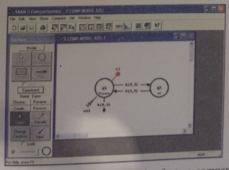
The figure above shows the SAAM II interface along with a two compartmental model containing an essential plasma compartment and a swap compartment. The SAAM II principle for the transfer coefficients is represented as k (i, j). Based on this illustration, k (2, 1) is the transfer rate to compartment 2 from compartment 1. Similarly, k (1, 2) is the transfer rate to compartment 1 from compartment 2. On the other hand, k (0, 2) is the rate of irreversible loss from compartment 1. In the diagram above, a toolbox is illustrated on the left-hand side of the window. This toolbox indicates model building and experiment building tools. With the use of these tools, the user can be able to sketch the compartments on the drawing canvas to indicate the movement from one compartment to another. Similarly, the toolbox can aid in initiating delays when required and coming up with experiments and samples that link to the data samples gathered.
In SAAM II, experiments are required to replicate the performance of the model. The EX1 is an experiment generated in the model through which the exogenous input in it is stated directly. On the other hand, S1 stands for a sample site. Notably, each entity represented on the illustration canvas has a related dialog box. These boxes can hold compartments’ reference names, input type and initial amount, measurement equations. Similarly, these boxes are where models can be associated with a detailed data set. As such, the information is fed independently in data tables from outside data files or developed internally. At last, parameter values are fed using the parameter entry dialog box.
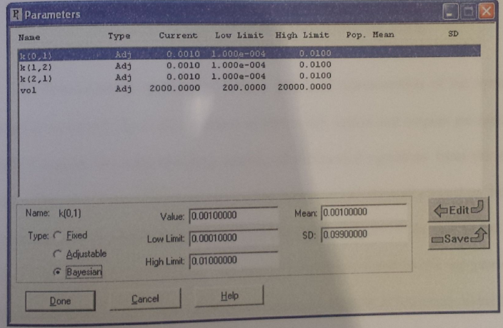
The parameter window’s function is to record all the parameters in the model together with their values and types, such as fixed, adjustable, or Bayesian. An example of a parameter window is illustrated in figure 2 below. In SAAM II, parameters represent those variables appearing in equations without and are not explicitly defined. Therefore, the user is free to modify the parameter’s type value and its high and low limits contained in the boxes situated underneath the dialog box. Thereafter, the user should keep the entries in the parameter list. Customized parameter values can be helpful when optimization is being carried out as they provide optimal fits to the data. When the Bayesian check box in computational settings is chosen, mathematical functions such as the population mean and SD come into appearance.
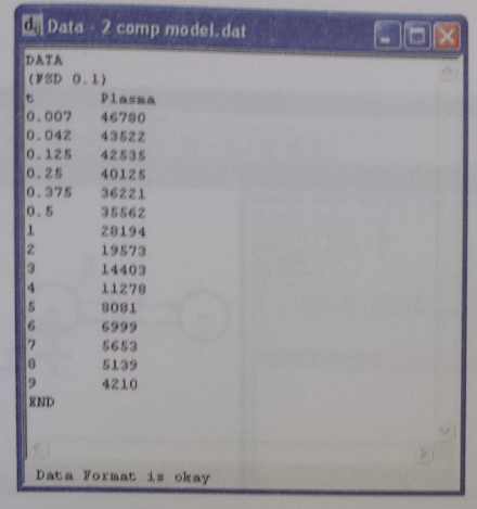
Another important facet of SAAM II is the data window. Data window utilizes tables in a specific format, which enables combinations of values, weighting, and un-weighting for particular data elements. Notably, data are listed in numerous columns with connected column titles, contained in a single or more table. An example of a data window is shown in figure 3 below.
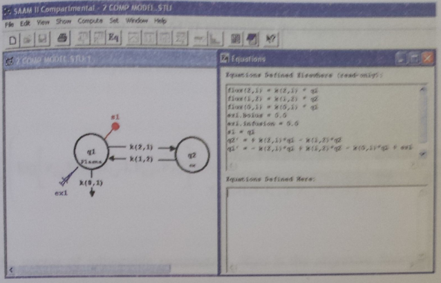
Compartmental models are graphical representations of differential equations systems. After the arrangement of the model, data fed, and outputs have been identified, SAAM II generates the matching differential equations out of the model structure. Figure 4 below illustrates equations generated internally by SAAM II in accordance with the two compartmental model structures. Similar equations can be specified by the user in the lower window indicated in figure 4. Note that the equations indicated in the uppermost part of the window are the key differential equations integrated numerically by SAAM II. Whenever a user works out a compartmental model, SAAM II integrates these differential equations illustrating the model throughout the period of the experiment with the help of the current parameter values. Equally, during this period SAAM II solves related algebraic equations.
On every occasion that SAAM II is initiated to fit a model to a data, it calls the optimizer. By use of a series of iterations, SAAM II alters the values of specific user allowed parameters in order to obtain the ideal fit among the calculated values, the data, and Bayesian prior information. During the optimization process, three values are put into consideration. These values are a total objective function, Akaike information criterion, and the Schwarz-Bayesian information criterion. The total objective function is reduced during the process and the two information criteria. On the other hand, the Akaike information criterion and the Schwarz-Bayesian information criterion can be used in the evaluation process of the model order. During this process, the model with the least value is considered appropriate. The iterative process is maintained up to the level where SAAM II’s convergence criteria, such as internal measures of the goodness of the fit, are met. Consequently, the process can be maintained up to the level where the maximum number of iterations specified has been attained.
Total objective function
In order to attain the best fit, SAAM II should reduce the objective function as indicated in figure 5 below.

Figure 5: the total objective function formula
From the above equation, p is the vector of modifiable parameters. R (p) is the objective function, while m p, k is the mean value of p, k over a cluster of analogous subjects or population mean. On the other hand, σ p, k is the standard deviation pk in a given population. Yi, j is the ith data in the jth data set. S (p, ti, j) is the model value. A sample in the compartmental module equivalent to yi, j at the time tI, j, v j is the variance parameter in the jth data set. Vi, j(s (p, tI, j), yi, j vj) is the variance model for yi, j where j is the number of data sets. Finally, m is the total number of data points.
Apart from indicating the value of the objective function, the statistics window also indicates the value of the Akaike information criterion and the Schwarz-Bayesian information criterion. The Akaike information criterion, as compared to other related methods, offers easy and efficient methods of the relative goodness of fit of a statistical model. A renowned scientist by the name Hirotsugu Akaike created this criterion in the early 1970s. The criterion is normally defined using the formula AIC= -2log (L) +2K. In this equation, K represents the number of parameters in the statistical model, whereas L represents the maximized value of the probability function of the model. According to the general definition of this criterion, the goodness of fit is recompensed. Nevertheless, a consequence arises as a rising function of the numeral of parameters. In general, the criterion is an evaluation of an approximation of the probable relative distance between the fitted model and the true unknown mechanism, which created the observed data. Each time several candidate models are selected, an individual is expected to calculate AIC values for these models and pick the model that corresponds with the least AIC value. The model that corresponds with the least AIC value is selected because it is the next from other possible samples considered to the unknown reality the data were generated from. In this regard, AIC is very important during the selection of the best model in a given set. However, it should be noted that when all the models are deprived of quality, AIC will not indicate a forewarning of that. As such, AIC will pick the one considered the best regardless of its quality.
AIC values are generally positive. Nevertheless, when an additive constant shifts values, a negative value is obtained. A single AIC value in itself cannot be deduced because of the unidentified interval scale. Particularly, AIC is proportional to the other AIC values in the model set. The absolute size of the AIC value is not useful but rather its relative values over the set of models considered. To compute and present the AIC differences overall candidate models in a set, we use the formula ∆i= AIC-AICmin. It is deemed that models with ∆i>10 do not possess the necessary support. After analyzing the AIC dissimilarities, the user should find how big the dissimilarities matter. Using the following expression exp (-1/2∆i), the relative probability of the ith model reduces the approximated information loss (Burnham 54).
On the contrary, a Bayesian information criterion is an approach that is used in picking a model amid a limited number of models. Just like the AIC criterion, this criterion relies on the probability function. Owing to this, it is closely linked to the Akaike information criterion. Thus, it would not be analyzed separately from AIC values. When carrying out this application, a compartmental depiction of the NCRP 67 plutonium system model was generated with the help of SAAM II, as shown in figure 6 below.
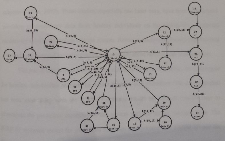
Equally, a sequence of SAAM II experiments was generated from the data collected from animals injected with intravenous. These were designed as a single bolus injection in the blood/plasma compartment. The amount of injection administered is indicated in the dialog box. Later, samples were generated in accordance with the available data linked to the data entered in a data table. Finally, parameter values were assigned to every transfer carried out in the compartments in accordance with the published transfer rates stated by ICRP 67, as shown in figure 6 above.
Conclusion
As earlier stated, simulation, analysis, and modeling software II is pharmacokinetic analysis software designed for studies of radioactive experiments. Employed internationally by more than 6,000 pharmaceutical, biomedical, and bioengineering experts and referred to in more than 1500 scientific journals, SAAM II is a confirmed and dominant instrument used in research, development, and education. The system provides assistance for the services of the biomedical problem through consultation on the use of the software and analysis and kinetic data. In addition, the model is user-friendly. As such, even with little expertise, an individual can be able to describe models, carry out some simulations, and scrutinize the findings with ease. To achieve its operations, the model makes use of high-tech numerical and statistical processes and algorithms. Compared with other related software, SAAM II has commonly considered the strongest and most precise software for resolving schemes of differential equations, which would otherwise seem difficult to solve in the absence of the package. Current research related to SAAM II will, in the future, improve the system’s efficiency and make the system more interactive (Burnham 123). There are two ways of creating these models (Burnham 123). These are by means of compartmental and numerical applications. For both methods for designing SAAM II models, simulation of complex experimental designs can be achieved. After designing the models, the user can then solve them before fitting them to the data with the help of special mathematical and statistical methods.
Works Cited
Burnham, Kenneth. Model selection and multimodel inference: a practical information-theoretic approach. 2nd ed. New York: Springer, 2002. Print.