Main Hypothesis and Nature of Relationship
For the testable hypothesis, we posit that sustained economic growth is a function of stable government (or rule of law), proximity to export markets, gross domestic investment, and an outward-looking economy. These are operationalized as follows:
- The effect or dependent variable is annual growth rate in per-capita income (G in the ACLP codebook).
- The first independent variable selected is the stability of government. In the codebook, this is “RSPELL: Number of successive spells of political regimes as classified by REG. A spell is defined as years of continuous rule under the same regime.” One expects an inverse relationship, anticipating that the fewer the spells, the more consistent are the laws and edicts that regulate business and therefore, the greater the chance that economic activity will flourish.
- For the second independent variable, geographic location matters because a nation that is just beginning to flex its muscles, so to speak, in international trade would benefit from lower costs of shipping to industrialized neighbor countries in North America, Europe or East Asia. On the other hand, robust importing demand is unlikely in South Asia or Latin America. The variable of choice is REGION because of the numerical values assigned to Southeast Asia and the OECD countries.
- The third variable is investment, operationalized as INV: Real gross domestic investment as a percentage of GDP at 1985 international prices. This is premised on the rationale that no economy can attain sustainable economic growth unless there is continuing public and private investment in infrastructure, educating the (future) labor force, in health care facilities, in new factories and R & D.
- Finally, the fourth variable is degree of participation in foreign trade. Expressed as “OPENC: Exports and imports as a share of GDP (both in 1985 international dollars)” inclusion is based on the rationale that, all other things equal, foreign trade gives a nation not only capital surpluses but also access to technology transfer.
Univariate Summaries
Table 1:
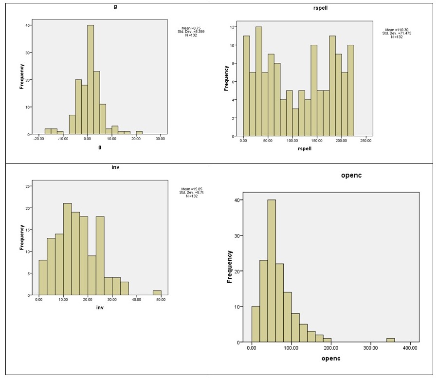
Over the four decades covered by the “Democracy and Development: Political Institutions and Material Well-Being in the World” database, annual economic growth adjusted for population sizes in the 132 countries has ranged from minus 17% to as much as 21.4% (see table above). The mean value of 0.75% implies a negative skew in the distribution (see also charts below) and that, on the whole, economic growth as measured by gross national product has expanded marginally faster than population growth. Globally, nations were not better off in 1990 than in 1950.
The first independent variable (IV), regime stability, is interesting for being bipolar. The calculated mean years of being ruled by the same regime, 110 years (see Table 1 above) is actually deceptive because most countries skew towards either highly stable rule (upwards of 150 years under either democratic or dictatorial rule, see Figure 1 below) or rapid transitions from one to the other.
The second IV, geographic location, is of course a static categorical variable since regional “affiliation” does not change over time. For the moment, univariate analysis of this variable can consist solely of counting the number of countries belonging to each. Table 2 reveals that the two regions of interest in this analysis, East Asia and the OECD member-nations, collectively comprise 42 countries or a shade under one-third of all nations.
Table 2: Distribution by Region
The third IV, real investment, ranged from 1% of gross domestic product to as much as 49%, though more typically at around 15% or 16%. This suggests wide disparities in resources that could be devoted to investment, as well differences in in the will of either the private or public sector (or both) to deploy those resources for fueling economic development.

As to the fourth IV, foreign trade in relation to gross domestic product was recorded at from 2.5% to 343.2% (Table 1). The realistic benchmark is the modal class interval of from 41% to 60% (see Figure 2) rather than the mean of 66% since the latter is unduly influenced by outliers (e.g. Singapore, Taiwan) that frequently achieve foreign trade totals twice or thrice their domestic product.
Relationships Between the Dependent and Independent Variables
We test for the existence, direction, and strength of the relationship with a combination of crosstabulation and scatterplots.
Table 3:
Given the categorical nature of REGION, a crosstab was tried with G recoded into class intervals. The result, Table 3, suggests that location within a trading region alone is inconclusive. First of all, 8 in 10 countries experienced low per-capita income growth (1% to 10%) or typically endured sluggish contractions (-1% to -10%) throughout 1950 to 1990. This is true for the OECD countries and, with one exception, those in East Asia. On the other hand, 10% of the Latin American and European countries outperformed the rest of the world by averaging 11% per-capita income improvement or better, albeit this really stands for just two countries. Hence, steady and satisfactory improvements in per-capita income were not the preserve of either the industrialized economies or Japan and the “little dragon” newly industrializing, export-oriented nations of East Asia. Plainly, other variables were at work besides proximity to robust trading partners.

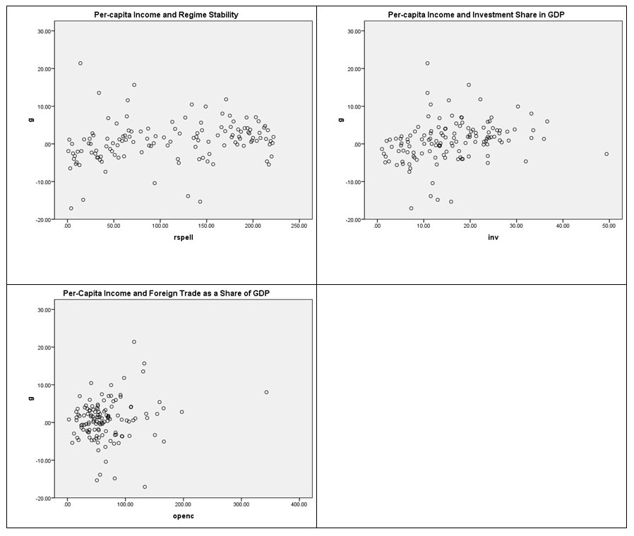
Visual inspection of Figure 2 above suggests that regime stability may have the weakest link to G among the three IV’s that were scale variables and could therefore be drawn on a scatter plot. The trend line would likely be perfectly flat (no relationship) and growth in per-capita income may continue to fluctuate slightly above or below zero regardless of how long a nation has remained under a democratic or dictatorial regime.
The openness of the economy in terms of foreign trade in relation to purely domestic output of goods and services (OPENC) may reveal a positive trend line. But this demands adjustment of the data and further manipulation because most of the data points cluster between 0% and 100% share to GDP. As first step, one would have to see what happens when the high share of GDP outliers are removed.
In contrast, the test of G against INV, real gross domestic investment as a percentage of GDP, has better potential for discovery of a positive relationship because: a) The scatter plot will accommodate a slightly sloped trend line; and, b) The data points are more satisfactorily dispersed from 0 (a negligible share) to around a 36% share of domestic investment in GDP. In fact, a preliminary stepwise regression run on all three IV’s (see Table 4) lends credence to a model where:
G = -3.01 + 0.10 (INV) + 0.02 (OPENC) + 0.01 (RSPELL)
INV brings about the largest change in G and a significance index better than 0.05 at the partial equations stage.
Table 4: Stepwise Regression Results:
Interpretation of the Relationship
Though INV gives the most grounds for optimism, the β value does not seem especially large. A good part of the explanation may lie in the fact that there is a lagged relationship between domestic investment and a favorable impact on per-capita income. After all, registering with the government a $1 million investment to build a factory this year impacts on domestic output many months or a year later. In national income accounting, increased output also equates with either savings or personal consumption expenditures (PCE) by the employees and suppliers of the new plant. Hence, the beneficial impact of the investment on family incomes eventuates some time later.
Alternate Hypotheses
On a global scale, in fact, per-capita income can be a misleading variable since it is derived by dividing the estimated value of domestic production of goods and services into the population that year. That per-capita figure masks many disparities across industrialized economies, the middle-income developing countries (MDCs), and the less developed countries. “Per-capita income” conceals inequity in income distribution among the upper-, middle- and low-income strata of a nation. An investigation into the antecedents of well-being should therefore consider income distribution as the DV at some stage. In the Codebook, this is the variable GINI, standing for the Gini ratio of income earned by the upper and lower extremes of the population.
- A second alternate hypothesis…
- Yet a third alternate hypothesis…
- Statistical Tests of Causal Hypotheses