Introduction
The research question to be answered is “What are the best predictors for the pulp quality?”
The Kappa number indirectly characterizes the content of residual lignin in a fibrous semi-finished product. It is determined by the volume of a potassium permanganate solution with a concentration of 0.02 mol / l consumed during titration per 1 g of absolutely dry cellulose (Correia et al., 2017). The chemical composition and physical and mechanical properties of cellulose depend on the wood species and manufacturing conditions. Chemical composition is the main factor determining the yield of cellulose, behavior during further processing (for example, during bleaching), as well as color and strength indicators. The properties of technical cellulose depend not only on the morphological structure of the fiber, but also on the reactions occurring with polysaccharides in an alkaline medium and the degree of delignification.
The content of residual lignin (expressed in permanganate units, for example such as a Kappa number) determines the direction of cellulose use. It can be either unbleached or bleached type to produce paper for printing. In this paper, it is investigated how the Kappa number can be used to estimate the lignin content in fibrous semi-finished products by an indirect method. To do this, scientists take into account the specific relationship between the number of Kappa and the lignin content for each type of semi-finished product.
Description of the Data
This data set was collected hourly over eight months under closed-loop control from Kamyr pulp digester of Weyerhauser city in western Canada province Alberta (Correia et al., 2017). 301 observations of 22 process measurements are included in it. All the varieties belong to the continuous type (Choi & Kwon, 2019). There are several ways to deal with the missing values. The author deleted all the missing values in this project and was left with 132 extensive observations (Choi & Kwon, 2019). The outliers checking was performed with Cook’s distance that computes the influence exerted by each data point row on the predicted outcome. There were three outliers, and the author deleted these three observations and was left with 129 observations.
The relationship between the variables was indeed detected with the help of Multivariate Multiple Linear Regression (Correia et al., 2017). It is a statistical test used to predict multiple outcome variables using one or more other variables. It also is used to determine the numerical relationship between these sets of variables and others. The variable one wants to predict should be continuous, and one’s data should meet the other assumptions listed below. First, the author checked the four assumptions, and the data met all the necessary criteria. It was normally distributed, independent, not linear, and had constant variance.
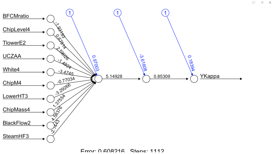
The author then checked the scatterplot to see the relationship between each predictor with the response. They detected that some of the predictors have a very weak relationship. The following research step selection method was employed to get the important predicted variables. Among them was the classical variable selection method, which is stepwise selection. The significant predictors were BFCMratio, ChipLevel4, TlowerE2, UCZAA, White4, ChipM4, LowerHT3, ChipMass4, BlackFlow2, and SteamHF3 (Choi & Kwon, 2019). The treatment of interest for this project are included Kappa Number or degree of delignification (“YKappa”) as a response, the active alkali of liquor in the upper cook zone (“UCZAA”), BFCMratio, ChipLevel4, TlowerE2, White4, ChipM4, LowerHT3, ChipMass4, BlackFlow2, and SteamHF3.
During checking the correlation between the variables with the correlation matrix, some weak relationships were detected. Then multivariate linear regression was repeated with the ten predictors, and the assumptions were checked. Still, there was no improvement in the assumptions. The data was still normally distributed, independent, non-linear, and had constant variance. The author tried to make the data linear and did two transformations on the response “YKappa.” First, using square root (YKappa), they checked the assumptions, and still, it was non-linear. Secondly, log (YKappa) was used (Correia et al., 2017). However, it did not improve the assumptions, and it was still a non-linear result. In this case, the author decided to do a Non-Linear Regression analysis.
Proposed Analyses
The method used in addressing the research interests is Regression Artificial Neural Network (ANN). It is the first generally accepted step for anyone who enters the field of Deep Learning. Inspired by the structure of the Natural Neural Network present in the human body, ANN mimics a similar structure and learning mechanism. ANN is an algorithm to build an efficient predictive model. Since the algorithm and its implementation resembles a typical neural network, it is named so. First, a neural network in R programming that solves a regression problem was constructed (Kumar, 1999). Before uploading the data into a neural network, it is good practice to perform normalization. There are several ways to perform normalization. In this research, the min-max method and scale of the data in the interval [0,1] will be used (Choi & Kwon, 2019). The data is then split into training (80%) and testing (20%) sets.
After that, a neural network using the neural net library can be created. Then the parameters are modified and the mean squared error (MSE) is calculated. The parameters selected for further use contain the least MSE. The author then uses two hidden layers having 1 and 1 neurons. After that, they utilize two hidden layers having 2 and 2 neurons, and then – two hidden layers having 3 and 2 neurons (Correia et al., 2017).
However, modifying and testing the neural network, again and again, is the best way to find the parameters that best fit the present model. When this neural network is trained, it will perform gradient descent to find coefficients that fit the data until it arrives at the optimal weights (in this case regression coefficients) for the model. Then the author compared the four neural networks with different layers and compared the MSE:
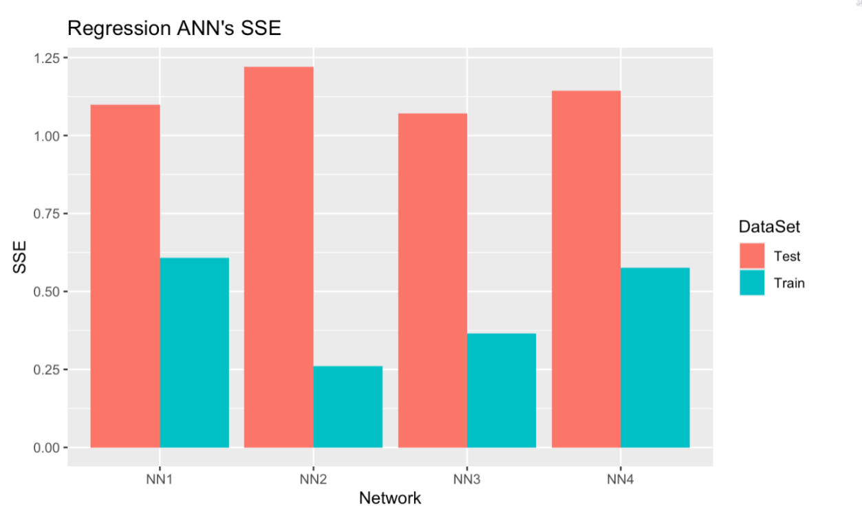
As can be seen in the table, there is no correct value for MSE. That means that the lower the value the better and 0 means the model is perfect (Correia et al., 2017). In this case, it can be seen that Neural network (1) has the smallest MSE. The author will also compare the test error to the training error for each Neural Network, to see the difference. From the plot below the comparison can be seen. The best result is when the training SS Error is approximately close to the testing SS error.

Analysis Results
The results of analyzing the data were received using Neural Network. With a single layer of output nodes, the author had a small MSE which was equal to 001063657 (Kumar, 1999). By comparing the two SSE, it can be seen that they are approximately close. The training SSE is equal to 1.099015, whilst the testing SSE is equal to 0.608 (Kumar, 1999). The Neural Network model plot will be later changed for the one which suits the research question better.

Conclusions
The best predictors for the pulp quality are BFCMratio, ChipLevel4, TlowerE2, UCZAA, White4, ChipM4, LowerHT3, ChipMass4, BlackFlow2, and SteamHF3.
References
Choi, H. K., & Kwon, J. S. (2019). Multiscale modeling and control of Kappa number and porosity in a batch-type pulp digester. American Institute of Chemical Engineers Journal, 65(6), 165-179.
Correia, F. M., d’Angelo, H. V., Almeida, G. M., & Mingoti, S. A. (2017). Predicting Kappa number in a Kraft Pulp continuous digester: A comparison of forecasting methods. Brazilian Journal of Chemical Engineering, 35(3), 1081-1094.
Kumar, S. (1999). Application of multivariate analysis techniques in understanding complex industrial processes: A Pulp Mill example. Web.