Economic Variables for the UAE: Mathematics and Statistics Report (Assessment)

Introduction

Statistics is an important area of study because it gives direction on how to record data, code, process, and analyze data. Besides, it is used in various fields such as medicine, business, science, and psychology because there are numbers involved in these areas. This project under mathematics and statistics will focus on analyzing some economic variables for the United Arab Emirates. The variables that will be analyzed are gross domestic product, inflation, and population. Further, descriptive statistics, charts, and regression are the statistical tools that will be used to analyze the data.

The objective of the Paper

The key objective of this paper is to make use of a number of statistical tools to analyze and understand various economic variables. In addition, the paper will also make use of graphs and charts to display the data collected.

Search of Data

The entire data will be obtained from the internet. Specifically, the data will be drawn from the International Monetary Fund website (International Monetary Fund, 2017). The website generally contains a variety of macroeconomic data series for most countries of the world. Some of the data that are available on the website are inflation, gross domestic product, unemployment, and government spending, among others. The website is updated on a regular basis, and it contains reliable economic statistics for various countries. The data for the three variables will cover the period between 1980 and 2016. The data are summarized in the table below.

Table 1: Data. Contains data for the three variables. (Source of data – International Monetary Fund, 2017).

Method of Analysis

The data is analyzed using various functions and formulas in Microsoft Excel 2010. First, scatter diagrams, column graphs, and histograms will be used to display the data. This can be found in the charts icon that is under the insert function in Excel. Secondly, descriptive statistics and regression analysis will also be used to study the data. This can be done using the data analysis tool that can be found under the data function.

Results and Discussion

Gross Domestic Product (GDP)

Table 2: Descriptive statistics. The table contains the mean, minimum, maximum, range, and standard deviation for GDP.

The average value of GDP is AED640.05 billion, while the standard deviation is AED301.02 billion. The median value is AED549.92 billion. The minimum value is AED270.117, while the maximum is AED1217.02. This yields a range of AED946.90 billion. Further, the kurtosis is less than 3. This implies that the data does not follow a normal distribution. Also, skewness is 0.4869, and it shows that the data is not symmetrical. It is moderately skewed. The scatter plot diagram for GDP is displayed below.

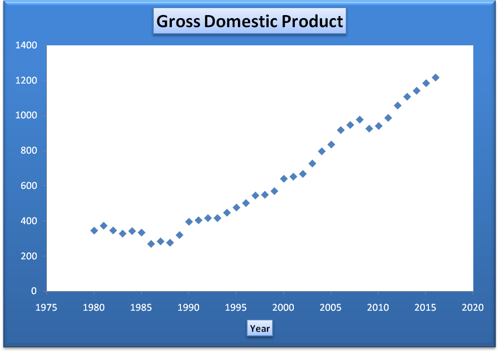
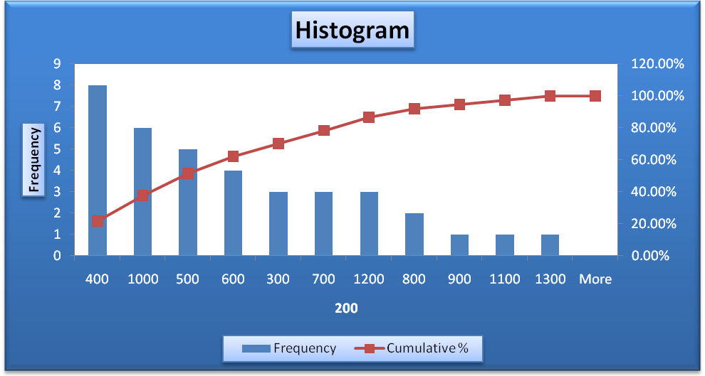
There is a clear upward trend in the graph. It shows that the GDP has been increasing over the years. However, it can be noted that between 1986 and 1989, the country experienced a slight decline in GDP. The country also experienced a slight drop in 2009. This was majorly caused by the global economic recession (International Monetary Fund, 2017). One major factor that has caused a tremendous growth in GDP is the income generated from the sale of oil. The country is an oil-producing nation. The results for a histogram are presented below.

Table 3: Histogram. It shows the frequency and the cumulative frequency that is used to construct the histogram.

Inflation

Table 4: Descriptive statistics. The table contains the mean, minimum, maximum, range, and standard deviation for inflation.

The average inflation, as measured using the consumer price index, is 159.61. The standard deviation is 65.14. The median index is 138.1. The minimum value of the index is 66.7, while the maximum value is 270.36. This yields a range of 203.662. The value of kurtosis is -1.1172. It is less than 3, and it shows that the data does not follow a normal distribution. Also, the value of skewness is 0.5286. It indicates that the data is moderately skewed to the left. This implies that the data is not symmetrical. The scatter plot diagram for inflation is displayed below.

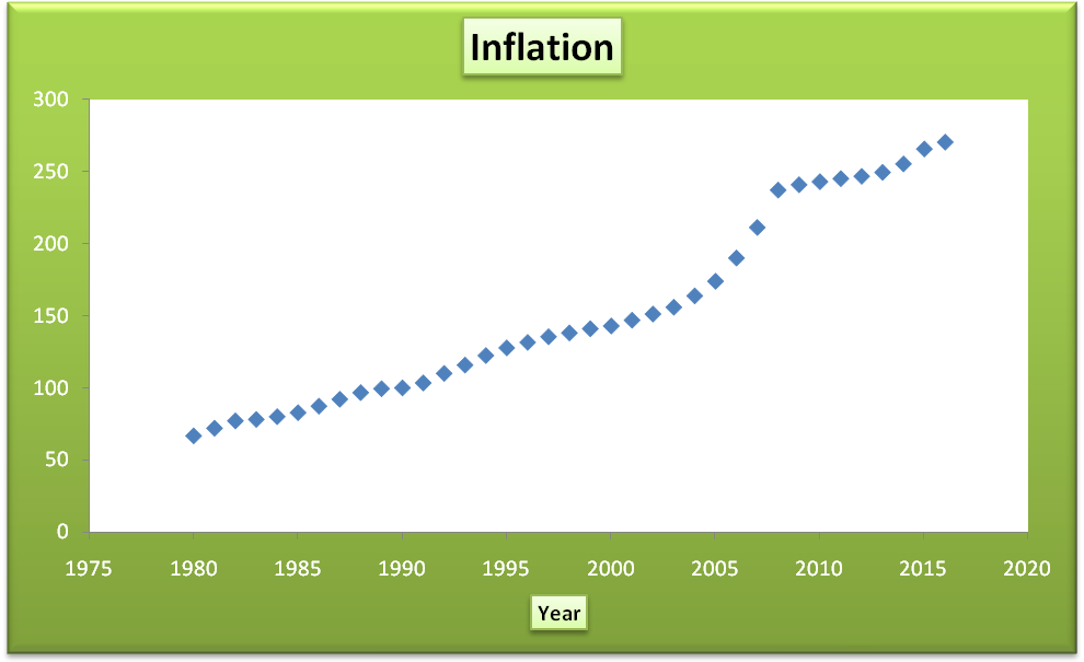
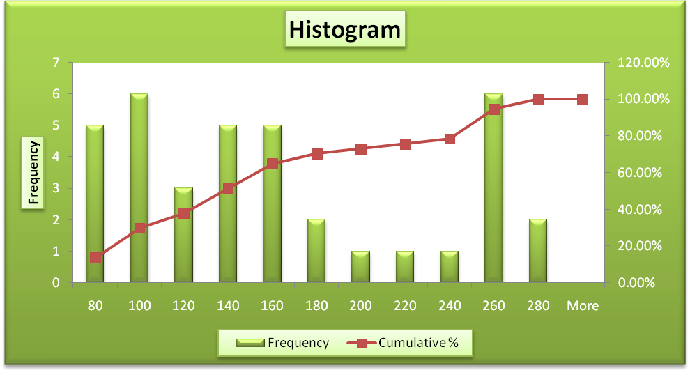
In the graph, it can be noted that there was an upward trend in the values of inflation. It shows that the country experienced general price increases. The growth rate of inflation was high during the global recession period (Bulmer, 2012). During the 37 year period, the inflation in the country grew by about 4 times. The histogram for inflation is displayed below.

Table 5: Histogram. It shows the frequency and the cumulative frequency that is used to construct the histogram.

Population

Table 6: Descriptive statistics. The table contains the values of inferential statistics.

The average population for the United Arab Emirates is 4.024 million people. The median and the standard deviation are 2.8 and 2.9, respectively. The kurtosis is -0.805. It shows that the peak of the data is shorter and broader than that of a normal distribution. The minimum value of the population is 1.01 million, while the maximum value is 9.89 million. This yields a range of 8.846 million. The bar graph below gives a pictorial representation of the trend of the population over the year.

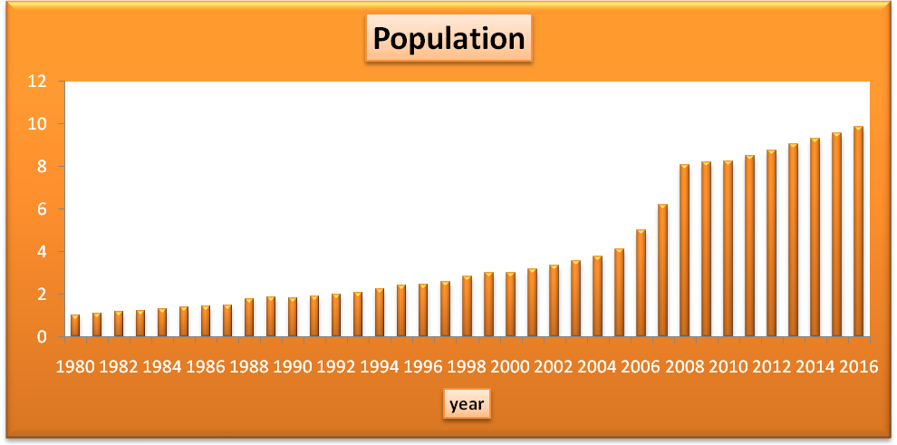
In the graph, it can be noted that there has been a continuous growth of population in the country. Between the years 2005 and 2008, the country experienced tremendous growth in population. Thereafter, the population increased at a low rate.

Simple Regression – Relationship between GDP and Inflation

This section will focus on using statistical tools such as correlation and regression to evaluate the relationship between the two variables. Inflation and GDP are two significant variables in an economy. Besides, some growth in GDP is often attributed to inflation. Therefore, this analysis will focus on establishing whether there is an association between the two economic variables. The table below shows the correlation results.

Table 7: Correlation results.

The correlation between GDP and inflation is 0.977. The value is close to one, and it indicates that there a perfect positive correlation between the two variables. Correlation does not indicate causality. Thus, it cannot be stated that one variable causes the other to increase. However, it shows that the variables move in the same direction. If one variable increases, then the variable is likely to increase. Another statistical tool that will be used in the analysis is regression. The results are displayed below.

Table 8: Regression results.

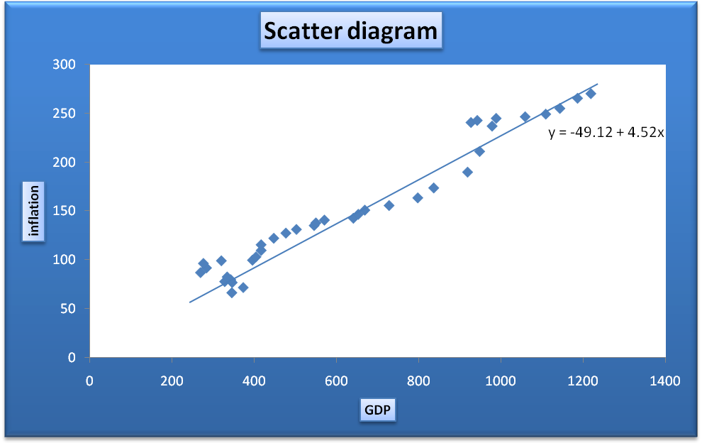
The regression equation will take the form Y = a + bX, where Y and X represent GDP and inflation, respectively. Based on the results, the regression equation will be Y = -49.12 + 4.52X. Intercept is -49.12. It has no significant statistical interpretation. It simply shows the variables that have not been included in the regression equation. The coefficient value is 4.52. The value is positive, and it implies that there a positive relationship between GDP and inflation. This implies that if inflation increases by one unit, then GDP is expected to increase by 4.52. The coefficient of determination (R-square) is 0.9547. The value shows that 95.47% of the variations in GDP are explained by changes in inflation. It is an indication of a strong explanatory variable (Fraser, 2012). The value of an adjusted R-Square is also high at 0.9535.

Another area that can be analyzed in the regression results is the significance of the explanatory variable. This can be done by looking at the p-value and t-statistic. From the table, the t-statistic for inflation is 27.1739, while the p-value is 4.08E-25. The p-value is less than the significance level of 0.05. This implies that inflation is a significant determent of GDP at the 95% confidence level. Evaluating the significance of the intercept is not necessary (Bulmer, 2012).

The final area that will be analyzed in the regression result is ANOVA. It is used to test the significance of the entire regression line. This will be achieved by evaluating the F values. From the table, F-statistic is 738.44, while the significance F is 4.08E-25. This value is lower than the significance level of 0.05. This implies that the overall regression line is significant at the 95% confidence level (Keller, 2012). Thus, the statistical analysis indicates that the regression is significant and can be relied upon. Thus, inflation is a strong determinant of GDP. The scatter diagram for the two variables is displayed below.

Multiple Regression – Relationship between GDP, Inflation and Population

This will focus on evaluating the relationship between one dependent variable and more than one explanatory variable. It is the most widely used regression analysis because a number of dependent variables are affected by several other variables. For instance, GDP is affected by factors such as national debt, consumer expenditure, investment, imports, government spending, and exports, among others (Wasserman, 2013). First, an evaluation of the correlation between the three variables will be carried out. The correlation results are shown below.

Table 9: Correlation results.

The results show that there is a strong positive correlation between population and GDP (0.9578) and between inflation and population (0.9844). The positive correlation implies that the variables are moving in the same direction. The regression results are shown below.

Table 10: Regression results.

With the addition of population as an explanatory variable, the new regression equation will be Y = -86.99 + 5.11X₁ -13.22X₂. X₂ in the equation represents the population. It can be observed that the population has a negative coefficient. This implies that if the population grows by one unit, then GDP is likely to drop by 13.22 units. The sign of the coefficient is not consistent with the correlation results. The coefficient of determination has increased slightly to 0.9553. The increase can be attributed to the addition of one variable. The value shows that 95.53% of the variations in GDP are explained by the changes in inflation and population. The p-value for the population is 0.5285. It is greater than the significance level of 0.05. This shows that population is not a significant determinant of GDP at the 95% confidence level. It can be noted that despite the addition of population, inflation is still a significant determinant of GDP. The overall regression line is still significant because the value of significance F (1.14E-23) is less than the significance level of 0.05 (Wasserman, 2013).

A comparison between the simple and multiple regression results shows that the addition of an extra variable improves the value of the coefficient of determination. Therefore, in order to have a strong regression equation, it is important to include as many explanatory variables as possible and eliminate those that are not significant. In addition, a number of tests can be carried out to ascertain if the regression equation meets various thresholds such as normality, and homoscedasticity among others (Wasserman, 2013).

Conclusion

The paper focused on using statistical tools to analyze three economic variables. The economic variables are GDP, inflation, and population of the United Arab Emirates. The data for these variables are available on the International Monetary Fund website. The data cover the period between 1980 and 2016. The analysis first focuses on calculating the descriptive statistics for the three variables. In addition, scatter diagrams, histograms, and column graphs are used to display the trend of the data. The second part of the analysis focuses on the use of regression and correlation to evaluate the relationship between the three variables. The results show that there is a strong positive relationship between the three variables. In addition, inflation is a significant determinant of GDP, while the population is not a significant determinant at the 95% confidence level. Also, the two regression equations are statistically significant at the 95% confidence level. Finally, a comparison of the simple and multiple regression equations shows that the addition of more variables increases the explanatory power of the independent variables.

References

Bulmer, M. G. (2012). Principles of statistics (3^rd ed.). North Chelmsford, MA: Courier Corporation.

Fraser, C. (2012). Business statistics for competitive advantage with excel 2010: Basics, model building, and cases (2^nd ed.). New York, NY: Springer Science and Business Media LLC.

International Monetary Fund. (2017). World economic outlook database, April 2017. Web.

Keller, G. (2012). Statistics for management and economics (9^th ed.). Mason, OH: South-Western Cengage Learning.

Wasserman, L. (2013). All of statistics: A concise course in statistical inference (3^rd). New York, NY: Springer Science and Business Media LLC.