Forecasting Techniques Principles and Practices – Finance Report

Exclusively available on Available only on IvyPanda® Written by Human No AI

Abstract

Forecasting is an essential input to the decision-making process in an organization because the output of predictions is used to plan for the future. Due to the significance of forecasting, there have been a number of techniques that can be used to carry out different types of forecasts. This paper carries out forecasting using three techniques. Quarterly sales data for a period of five years is used in the estimation.

The specific methods that were used are forecasts based on analyst opinion, 3-period moving average, 4-period weighted moving average, and linear regression analysis. All three methods yielded different results. Analysis of the errors shows that the forecasts that were based on analyst opinion have the least MAD and MSE while the regression model had the least MPE. Therefore, the model that will best suit this situation is regression analysis.

Introduction

The concept of forecasting is quite important in an organization because every decision that is made now requires some prediction of their impact on the future. Some of the areas that companies usually focus on are the demand for the commodity, sales, and costs. Due to the increasing intricacy of the forecasting problem, there have been a number of techniques that have been developed.

These techniques have different uses, and it is necessary to correct the right method for a specific application (Chambers, Mullick & Smith, 2014). This paper seeks to discuss common forecasting techniques. Quarterly sales data will be used to demonstrate these techniques. The data will be for a period of five years, that is, between 2000 and 2004.

Discussion

Analysis of the original data

As mentioned above, the sales revenue data are for a period of five years, which is between 2000 and 2004. The data are arranged in quarters. The table below shows the historical data of sales revenue for the company for various periods.

Historical Sales Revenues
YearQuarterPeriodSales
200011$684.20
200022$584.10
200033$765.40
200044$892.30
200115$885.40
200126$677.00
200137$1,006.60
200148$1,122.10
200219$1,163.40
2002210$993.20
2002311$1,312.50
2002412$1,545.30
2003113$1,596.20
2003214$1,260.40
2003315$1,735.20
2003416$2,029.70
2004117$2,107.80
2004218$1,650.30
2004319$2,304.40
2004420$2,639.40

The table shows that there has been a general increase in the sales revenue for the company for the five year period. However, the revenue generated from sales is cyclic, that is, it is low during the second quarter and increased gradually in the third, fourth, and the first quarter for all the years. The graph below shows the trend in sales revenue for the 20 periods in the five year period.
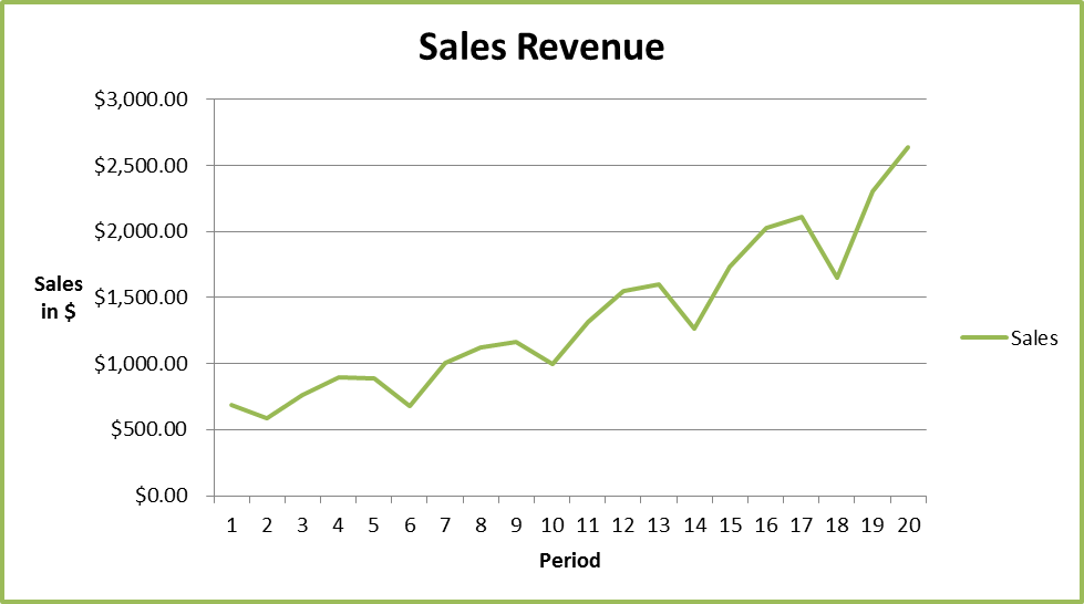
Sales revenue

The data on sales in quarters are presented below.

Quarter 1Quarter 2Quarter 3Quarter 4
2000$684.20$584.10$765.40$892.30
2001$885.40$677.00$1,006.60$1,122.10
2002$1,163.40$993.20$1,312.50$1,545.30
2003$1,596.20$1,260.40$1,735.20$2,029.70
2004$2,107.80$1,650.30$2,304.40$2,639.40

Forecasting techniques

There exist three basic categories of forecasting techniques. The three techniques are qualitative techniques, time series analysis and projections, and casual models. These three techniques use different approach to predict future values and they are discussed in the subsequent section.

Qualitative techniques

This technique is based on judgments and views of experts and available information on special occasions. This may or may not take into account historical trends. The data can be obtained through a number of ways. The first approach is by informing the salespersons to gather the sales data for different categories and time periods. Secondly, it is by getting the information from different employees at different levels. The third approach is by conducting customer surveys.

The customers can be contacted via a phone call or by using forms (Sandford & Hsu, 2007). The final way of obtaining such data is monitoring the sales of other related products such as complements and substitutes. A review of the opinions of the analysts shows that the sales value of the commodity will continue to rise in the same trend (Hyndman & Athanasopoulos, 2014). The table presented below shows the forecasted sales values using analysts’ opinions.

YearQuarterPeriodSalesForecasts
200011$684.20$694.46
200022$584.10$592.86
200033$765.40$776.88
200044$892.30$905.68
200115$885.40$898.68
200126$677.00$687.16
200137$1,006.60$1,021.70
200148$1,122.10$1,138.93
200219$1,163.40$1,180.85
2002210$993.20$1,008.10
2002311$1,312.50$1,332.19
2002412$1,545.30$1,568.48
2003113$1,596.20$1,620.14
2003214$1,260.40$1,279.31
2003315$1,735.20$1,761.23
2003416$2,029.70$2,060.15
2004117$2,107.80$2,139.42
2004218$1,650.30$1,675.05
2004319$2,304.40$2,338.97
2004420$2,639.40$2,678.99

Time series analysis and projections

Time series analysis makes use of the historical data to predict future values. The most common techniques that can be used under this category are moving average, linear regression analysis, trend estimation, growth curves, and exponential smoothing (Madura, 2014). Under this category, two methods will be used. They are discussed below.

3-period moving average

The table presented below shows results for the three-period moving average.

YearQuarterPeriodSales3-period moving average forecasts
200011$684.20
200022$584.10
200033$765.40677.90
200044$892.30747.27
200115$885.40847.70
200126$677.00818.23
200137$1,006.60856.33
200148$1,122.10935.23
200219$1,163.401,097.37
2002210$993.201,092.90
2002311$1,312.501,156.37
2002412$1,545.301,283.67
2003113$1,596.201,484.67
2003214$1,260.401,467.30
2003315$1,735.201,530.60
2003416$2,029.701,675.10
2004117$2,107.801,957.57
2004218$1,650.301,929.27
2004319$2,304.402,020.83
2004420$2,639.402,198.03

4-period weighted moving average

The table presented below shows results for the four-period weighted moving average.

YearQuarterPeriodSalesweightsSales * weights4-period weighted moving average forecasts
200011$684.200.2$136.84
200022$584.100.1$58.41
200033$765.400.3$229.62
200044$892.300.4$356.92$781.79
200115$885.400.2$177.08$822.03
200126$677.000.1$67.70$831.32
200137$1,006.600.3$301.98$903.68
200148$1,122.100.4$448.84$995.60
200219$1,163.400.2$232.68$1,051.20
2002210$993.200.1$99.32$1,082.82
2002311$1,312.500.3$393.75$1,174.59
2002412$1,545.300.4$618.12$1,343.87
2003113$1,596.200.2$319.24$1,430.43
2003214$1,260.400.1$126.04$1,457.15
2003315$1,735.200.3$520.56$1,583.96
2003416$2,029.700.4$811.88$1,777.72
2004117$2,107.800.2$421.56$1,880.04
2004218$1,650.300.1$165.03$1,919.03
2004319$2,304.400.3$691.32$2,089.79
2004420$2,639.400.4$1,055.76$2,333.67

Causal models

This category makes use of extremely advanced and exact information about the association between the variables. These models take into account particular occasions. In this case, the regression model will be used.

Linear regression model

Regression analysis is a statistical tool that is used to develop approximate linear relationships among various variables. Regression analysis formulates an association between several variables. There are a number of variables that can affect the sales revenue of a company. Some of the factors are the price of the products of the company, competition, news about the company, and the amount spent on advertising, among other factors.

When coming up with the simple linear regression model, it is necessary to separate between dependent and independent variables (Wang, 2010). In this scenario, the dependent variable is the sales revenue, while the independent variable is the time period.

The regression line will take the form Y = b0 + b1X

Y = Sales revenue

X = Time

The theoretical expectations are b0 can take any value and b1 > 0 (positive).

Regression Results

Regression Statistics
Multiple R0.934139098
R Square0.872615854
Adjusted R Square0.865538957
Standard Error215.1057043
Observations20
ANOVA
dfSSMSFSignificance F
Regression15705373.4975705373123.30491.74093E-09
Residual18832868.352446270.46
Total196538241.85
CoefficientsStandard Errort StatP-valueLower 95%
Intercept375.175789599.923366033.7546350.001451165.2445875
Period92.62563918.34144143111.104271.74E-0975.10092095

From the above table, the regression equation can be written as Y = 375.1758 + 92.62564X. The intercept value of 375.1758 represents other variables that affect the average sales revenue but are not included in the modeling. The coefficient value of 92.62564 implies that as time increases by one unit, the sales revenue increases by 92.6256 units. When the regression equation is compared with the scatter diagram, there is an indication of consistency.

The graph of average sales revenue and time shows an upward trend with a correlation coefficient of 0.9341. The regression equation above also yields a positive slope. The p-value for t-statistic is greater than α = 0.05. This shows that the variable is statistically significant. The overall regression line is also significant, as indicated by significance f in the ANOVA analysis.

Finally, the time period explains significant variations in the variation of sales, as indicated by the value of R-Square and adjusted R-Square. Thus, it is clear that the regression equation is sensible and can be used for forecasting. The graph below shows the graph of the original plots of sales revenue and time with a line of best fit.
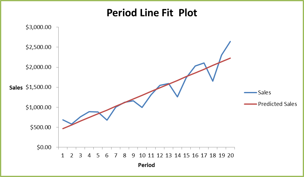
Period line fit plot

The table presented below shows the forecasted values of sales using the estimated regression model.

YearQuarterPeriodSalesRegression forecasts
200011$684.20467.80
200022$584.10560.43
200033$765.40653.05
200044$892.30745.68
200115$885.40838.30
200126$677.00930.93
200137$1,006.601023.56
200148$1,122.101116.18
200219$1,163.401208.81
2002210$993.201301.43
2002311$1,312.501394.06
2002412$1,545.301486.68
2003113$1,596.201579.31
2003214$1,260.401671.93
2003315$1,735.201764.56
2003416$2,029.701857.19
2004117$2,107.801949.81
2004218$1,650.302042.44
2004319$2,304.402135.06
2004420$2,639.402227.69

Evaluation of errors

In this section, three methods will be used to evaluate the errors in the forecasting techniques used in the subsequent sections.

Mean absolute deviation (MAD)

The results of the three methods are presented below.

Qualitative techniques

PeriodErrors
(Sales – forecast)
Absolute errors
1($10.26)10.26
2($8.76)8.76
3($11.48)11.48
4($13.38)13.38
5($13.28)13.28
6($10.16)10.16
7($15.10)15.1
8($16.83)16.83
9($17.45)17.45
10($14.90)14.9
11($19.69)19.69
12($23.18)23.18
13($23.94)23.94
14($18.91)18.91
15($26.03)26.03
16($30.45)30.45
17($31.62)31.62
18($24.75)24.75
19($34.57)34.57
20($39.59)39.59
Total absolute deviation404.33
Mean absolute deviation20.22

Time series analysis and projections

3-period moving average

PeriodErrors
(Sales – forecast)
Absolute errors
1$684.20684.2
2$584.10584.1
3$87.5087.5
4$145.03145.03
5$37.7037.7
6($141.23)141.23
7$150.27150.27
8$186.87186.87
9$66.0366.03
10($99.70)99.7
11$156.13156.13
12$261.63261.63
13$111.53111.53
14($206.90)206.9
15$204.60204.6
16$354.60354.6
17$150.23150.23
18($278.97)278.97
19$283.57283.57
20$441.37441.37
Total absolute deviation4,632.16
Mean absolute deviation231.61

4-period weighted moving average

PeriodErrors
(Sales – forecast)
Absolute errors
1$136.84136.84
2$58.4158.41
3$229.62229.62
4($424.87)424.87
5($644.95)644.95
6($763.62)763.62
7($601.70)601.7
8($546.76)546.76
9($818.52)818.52
10($983.50)983.5
11($780.84)780.84
12($725.75)725.75
13($1,111.19)1111.19
14($1,331.11)1331.11
15($1,063.40)1063.4
16($965.84)965.84
17($1,458.48)1458.48
18($1,754.00)1754
19($1,398.47)1398.47
20($1,277.91)1277.91
Total absolute deviation17075.78
Mean absolute deviation853.79

Causal models

Linear regression model

PeriodErrors
(Sales – forecast)
Absolute errors
1$216.40216.4
2$23.6723.67
3$112.35112.35
4$146.62146.62
5$47.1047.1
6($253.93)253.93
7($16.96)16.96
8$5.925.92
9($45.41)45.41
10($308.23)308.23
11($81.56)81.56
12$58.6258.62
13$16.8916.89
14($411.53)411.53
15($29.36)29.36
16$172.51172.51
17$157.99157.99
18($392.14)392.14
19$169.34169.34
20$411.71411.71
Total absolute deviation3078.24
Mean absolute deviation153.91

In the above results, it can be noted that the qualitative method has the least MAD. Therefore, it will be preferred to the other methods.

Mean squared error (MSE)

Qualitative techniques

PeriodErrors
(Sales – forecast)
errors squared
1($10.26)105.2676
2($8.76)76.7376
3($11.48)131.7904
4($13.38)179.0244
5($13.28)176.3584
6($10.16)103.2256
7($15.10)228.01
8($16.83)283.2489
9($17.45)304.5025
10($14.90)222.01
11($19.69)387.6961
12($23.18)537.3124
13($23.94)573.1236
14($18.91)357.5881
15($26.03)677.5609
16($30.45)927.2025
17($31.62)999.8244
18($24.75)612.5625
19($34.57)1195.085
20($39.59)1567.368
Total errors squared9645.499
MSE482.2749

Time series analysis and projections

3-period moving average

PeriodErrors
(Sales – forecast)
Errors squared
1$684.20468129.64
2$584.10341172.81
3$87.507656.25
4$145.0321033.7009
5$37.701421.29
6($141.23)19945.9129
7$150.2722581.0729
8$186.8734920.3969
9$66.034359.9609
10($99.70)9940.09
11$156.1324376.5769
12$261.6368450.2569
13$111.5312438.9409
14($206.90)42807.61
15$204.6041861.16
16$354.60125741.16
17$150.2322569.0529
18($278.97)77824.2609
19$283.5780411.9449
20$441.37194807.4769
Total errors squared1,622,449.57
MSE81,122.48

4-period weighted moving average

PeriodErrors
(Sales – forecast)
errors squared
1$136.8418725.19
2$58.413411.728
3$229.6252725.34
4($424.87)180514.5
5($644.95)415960.5
6($763.62)583115.5
7($601.70)362042.9
8($546.76)298946.5
9($818.52)669975
10($983.50)967272.3
11($780.84)609711.1
12($725.75)526713.1
13($1,111.19)1234743
14($1,331.11)1771854
15($1,063.40)1130820
16($965.84)932846.9
17($1,458.48)2127164
18($1,754.00)3076516
19($1,398.47)1955718
20($1,277.91)1633054
Total errors squared18,551,829
MSE927,591.5

Causal models

Linear regression model

PeriodErrors
(Sales – forecast)
errors squared
1$216.4046828.96
2$23.67560.2689
3$112.3512622.52
4$146.6221497.42
5$47.102218.41
6($253.93)64480.44
7($16.96)287.6416
8$5.9235.0464
9($45.41)2062.068
10($308.23)95005.73
11($81.56)6652.034
12$58.623436.304
13$16.89285.2721
14($411.53)169356.9
15($29.36)862.0096
16$172.5129759.7
17$157.9924960.84
18($392.14)153773.8
19$169.3428676.04
20$411.71169505.1
Total errors squared832,866.6
MSE41,643.33

In the above results, it can be noted that the qualitative method has the least MSE. Therefore, it will be preferred to the other methods.

Mean percentage error (MPE)

Qualitative techniques

PeriodErrors
(Sales – forecast)
Percentage error
1($10.26)1.50%
2($8.76)1.50%
3($11.48)1.50%
4($13.38)1.50%
5($13.28)1.50%
6($10.16)1.50%
7($15.10)1.50%
8($16.83)1.50%
9($17.45)1.50%
10($14.90)1.50%
11($19.69)1.50%
12($23.18)1.50%
13($23.94)1.50%
14($18.91)1.50%
15($26.03)1.50%
16($30.45)1.50%
17($31.62)1.50%
18($24.75)1.50%
19($34.57)1.50%
20($39.59)1.50%
Total percentage errors30.00%
MPE1.50%

Time series analysis and projections

3-period moving average

PeriodErrors
(Sales – forecast)
Percentage error
1$684.20-100.00%
2$584.10-100.00%
3$87.50-11.43%
4$145.03-16.25%
5$37.70-4.26%
6($141.23)20.86%
7$150.27-14.93%
8$186.87-16.65%
9$66.03-5.68%
10($99.70)10.04%
11$156.13-11.90%
12$261.63-16.93%
13$111.53-6.99%
14($206.90)16.42%
15$204.60-11.79%
16$354.60-17.47%
17$150.23-7.13%
18($278.97)16.90%
19$283.57-12.31%
20$441.37-16.72%
Total percentage errors-306.21%
MPE-15.31%

4-period weighted moving average

PeriodErrors
(Sales – forecast)
Percentage error
1$136.84-100.00%
2$58.41-100.00%
3$229.62-100.00%
4($424.87)-12.38%
5($644.95)-7.16%
6($763.62)22.79%
7($601.70)-10.22%
8($546.76)-11.27%
9($818.52)-9.64%
10($983.50)9.02%
11($780.84)-10.51%
12($725.75)-13.04%
13($1,111.19)-10.39%
14($1,331.11)15.61%
15($1,063.40)-8.72%
16($965.84)-12.41%
17($1,458.48)-10.81%
18($1,754.00)16.28%
19($1,398.47)-9.31%
20($1,277.91)-11.58%
Total percentage errors-373.73%
MPE-18.69%

Causal models

Linear regression model

PeriodErrors
(Sales – forecast)
Percentage error
1$216.40-31.63%
2$23.67-4.05%
3$112.35-14.68%
4$146.62-16.43%
5$47.10-5.32%
6($253.93)37.51%
7($16.96)1.68%
8$5.92-0.53%
9($45.41)3.90%
10($308.23)31.03%
11($81.56)6.21%
12$58.62-3.79%
13$16.89-1.06%
14($411.53)32.65%
15($29.36)1.69%
16$172.51-8.50%
17$157.99-7.50%
18($392.14)23.76%
19$169.34-7.35%
20$411.71-15.60%
Total percentage errors22.02%
MPE1.10%

In the above results, it can be noted that linear regression analysis has the least MSE. Therefore, it will be preferred to the other methods.

Conclusion

This paper carries out forecasting using three techniques; these are forecasts based on analyst opinion, 3-period moving average, 4-period weighted moving average, and linear regression analysis. The model that will be the most suitable in this scenario is a regression analysis because it has the least MPE, and it is also comprehensive.

References

Chambers, J., Mullick, S., & Smith, D. (2014). . Web.

Hyndman, R., & Athanasopoulos, G. (2014). Forecasting: principle and practice. USA: Otext.com.

Madura, J. (2014). International financial management. USA: Cengage Learning.

Sandford, B., & Hsu, C. (2007). The Delphi technique: making sense of consensus. Practical Assessment and Research Evaluation, 12(10), 1-8.

Wang, J. (2010). Business intelligence in economic forecasting: technologies and techniques. USA: IGI Global.

More related papers Related Essay Examples
Cite This paper
You're welcome to use this sample in your assignment. Be sure to cite it correctly

Reference

IvyPanda. (2020, May 1). Forecasting Techniques Principles and Practices - Finance. https://ivypanda.com/essays/forecasting-techniques-principles-and-practices-finance/

Work Cited

"Forecasting Techniques Principles and Practices - Finance." IvyPanda, 1 May 2020, ivypanda.com/essays/forecasting-techniques-principles-and-practices-finance/.

References

IvyPanda. (2020) 'Forecasting Techniques Principles and Practices - Finance'. 1 May.

References

IvyPanda. 2020. "Forecasting Techniques Principles and Practices - Finance." May 1, 2020. https://ivypanda.com/essays/forecasting-techniques-principles-and-practices-finance/.

1. IvyPanda. "Forecasting Techniques Principles and Practices - Finance." May 1, 2020. https://ivypanda.com/essays/forecasting-techniques-principles-and-practices-finance/.


Bibliography


IvyPanda. "Forecasting Techniques Principles and Practices - Finance." May 1, 2020. https://ivypanda.com/essays/forecasting-techniques-principles-and-practices-finance/.

If, for any reason, you believe that this content should not be published on our website, please request its removal.
Updated:
This academic paper example has been carefully picked, checked and refined by our editorial team.
No AI was involved: only quilified experts contributed.
You are free to use it for the following purposes:
  • To find inspiration for your paper and overcome writer’s block
  • As a source of information (ensure proper referencing)
  • As a template for you assignment
1 / 1