Introduction
The management of Highline Financial Services has to determine the demand for the services of this organization during the next four quarters. Several challenges should be considered. In particular, there is an oscillating pattern of demand. However, the available data are not sufficient for calculating seasonal relatives. Therefore, it is difficult to apply such techniques as the centered moving average or simple average methods. Nevertheless, other tools can be useful for making intuitive predictions. Overall, this forecast can have significant implications for the senior executives of this company. In particular, this information is necessary for determining the number of workers who should be hired or dismissed. Furthermore, it is possible that business administrators will need to change some of the current practices to increase the demand for the services.
Forecasting methods
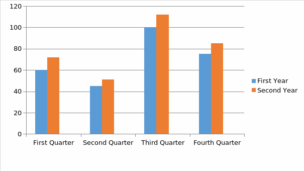
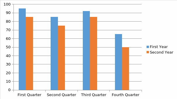
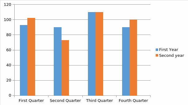
The changes in demand can be illustrated with the help of two bar charts because they can cast a light on the general trends affecting the company. In particular, one should focus on the quarterly changes in demand for during each year.


Overall, these charts indicate that there are certain seasonal variations. For instance, the demand for Service A declines during the second quarter, but it reaches the peak in the third quarter (Patnaik, 2015). This tendency has been observed during each of the two years. The variations of demand for Season B follow a similar pattern during the two years. However, the causes of these variations are not explained.
Moreover, one should note that the demand for Service B diminished consistently (Patnaik, 2015, p. 133). For instance, one can reach this conclusion by comparing corresponding quarters in each year. At the same time, the customers of this company became more willing to use Service A. Nevertheless, the level of demand for Service C fluctuates. It is one of the exceptions that should not be overlooked.
In this case, one can apply the so-called naïve forecast. This approach is premised on the assumption that the last indicator in the time series should be viewed as the basis for the prediction (Patnaik, 2015, p. 85). Furthermore, it is supposed that the difference between the last two values will be used to estimate the change in demand (Patnaik, 2015, p. 85). The forecast involves the comparison of corresponding quarters in each year. The results can be presented in the table format.
Table One: Service A.
Table Two: Service B.
Table Three: Service C.
This forecast is based on the additive approach to the estimation of demand. In this case, the person, who makes the prognosis, either adds or subtracts a certain quantity from the previous value (Patnaik, 2015). Admittedly, the naïve forecast is considered to be a very simplistic tool (Boyer & Rohit, 2009). This tool can yield valid results provided that the market trends do not change (Boyer & Rohit, 2009). Apart from that, the person has to assume that the changes of quantitative indicators will resemble an arithmetic progression, but it may follow a different pattern. However, this approach can be adopted if the time series is very short. Furthermore, this method is very time-efficient. So, this tool should not be disregarded.
The demand can also be estimated according to the multiplicative model. In this case, one should calculate the ratio of the second-year results to the first-year results. In turn, this coefficient will be applied to estimate the demand for the third year.
Service A.
Service B.
Service C.
Again, one should keep in mind that these estimates may not be accurate. The problem is that the results of the third year may not change according to the multiplicative model. It is one of the pitfalls that should be taken into account.
It is possible to consider such a technique as moving average. A manager should use the following formula:
- (Value1+ Value2 + Value3 +..+ Value n)÷n
In this case, one can compute the four-period moving average for each of the services offered by Highline Financial Services. In this case, the manager should pay attention to the most recent data because this information accurately reflects the latest trends in the industry (Chiulli, 1999). So, one should focus on the quarters of the second year.
- Service A
- (72+51+112+85) ÷4=80
- Service B
- (85+75+85+50) ÷ 4 =73.75
- Service C
- (102+75+110+100) ÷ 4 = 96.75
This method of forecasting will enable the management to estimate the level of demand for the first quarter of the third year. Admittedly, this approach does not take into account the possibility of seasonal variations. However, it is possible that this regularity may not exist. One should access a larger sample of data to show that the changes in demand can be explained by some seasonal or temporal changes. The problem is that random results can be confused with patterns and regularities if one looks at short time intervals (Chase, 2013). This possibility should also be considered by the management.
One can argue that the application of different forecasting techniques is helpful for estimating the range of demand during a given period such as 12 months. This knowledge is useful for determining the optimal number of employees who should be hired by Highline Financial Services in the future.
General trends and their implications
Although the forecasting methods can yield different results, they can illustrate some important tendencies. In particular, the demand for Service A has increased over the last two years, and it is possible that this trend will continue in the future. Additionally, the demand for Service B diminishes. In turn, it is difficult to make predictions about Service C. Thus, the management should spend more time to improve its operations. This argument is particularly relevant to Service B that does not appeal to many customers. However, it is possible that this trend cannot be attributed to internal weaknesses of the company.
For instance, this tendency can be explained by the changing needs of customers. In this case, the management should reduce the number of employees who work in this particular area. For instance, they can provide Services A and C. However, these recommendations can be elaborated if the managers collect data for a longer period. In this way, they can increase the precision of their forecasts.
Conclusion
Overall, this case suggests that business administrators should be skilled in using various forecasting methods. They need to understand the strengths and weaknesses of these tools. Furthermore, they should determine if the available data are sufficient for identifying certain patterns or regularities. For instance, it is possible to mention the existence of seasonal variations. In turn, the estimations included in this paper are based on the application of naïve forecasts, multiplicative models, and moving average.
These approaches are helpful for determining if customers will use the services of the company. Finally, one can argue that Service B should be the primary concern to the management. Moreover, business administrators should consider the results of forecasts to determine the optimal size of the workforce. This task is essential for reducing operational costs.
Reference List
Boyer, K., & Rohit, V. (2009). Operations and Supply Chain Management for the 21st Century. New York, NY: Cengage Learning.
Chase, C. (2013). Demand-Driven Forecasting: A Structured Approach to Forecasting. New York, NY: John Wiley & Sons.
Chiulli, R. (1999). Quantitative Analysis: An Introduction. New York, NY: CRC Press.
Patnaik, S. (2015). Operations Management. New York, NY: Lulu Press.