Introduction
Analyzing historical data of various countries is of essence since it gives trends of various variables for the past years. This can be used to used to estimate and forecast future values. Besides, the past trends can also explain future behaviors of various variables. The treatise carries out a comprehensive historical analysis of data for various countries.
It analyses the gross national product per capita of the countries. It carries out the analysis of the six regions provided. These are, Latin America, OECD, East Asia, ‘Other Asia’, Africa, and the Gulf. It compares the average gross national product per capita for the region. The paper further discusses the relationship between male life expectancy and female life expectancy.
Further, it discusses gross national product per capita in Africa in details. It also discusses the relationship between life expectancy of female and male. Finally, the paper carries out a regression analysis of the percentage of the adult literacy level of gross national product per capita.
Gross National Product (GNP) per capita
GNP per capita of each of the six countries will show the average value of goods and services produced by each individual in that nation. The value is arrived at by dividing the gross national product of the country by the total population of the country. The value is used to show the contribution of each individual to the growth of a nation.
Further, it also shows the living standards of people within a region. In most cases, well developed cities tend to have a higher GNP per capita than less developed nations. The first region is Latin America. It has a total of 21 countries with a total GNP per capita of 32,270. In the region, Trinidad and Tobago has the highest GNP per capita totaling to $3,610 per person.
Nicaragua has the lowest GNP per capita amounting to $360 per person. The average GNP per capita for the region is $1,536.67 while the range is $3,250. OECD region has 27 countries. The total GNP per capita for the region is $407, 020. Out of the 7 countries, Switzerland has the highest GNP per capita amounting to $32,370. Turkey has the lowest GNP per capita amounting to $1,640. The region has a big range amounting to $30,730. The average GNP per capita amounts to $15,074.81.
East Asia has 7 countries with a total GNP per capita amounting to $34,920. Singapore has the highest GNP per capita amounting to $12,400. Indonesia has the least GNP per capita amounting to $560. The range in the region is $11,840. The fourth region is ‘Other Asia’.
It has six countries with a total GNP per Capita amounting to $1,780.Sri Lanka has the highest GNP per capita amounting to $470 while Cambodia has the least GNP per capita amounting to $170. The range of the region is $300. The fifth region is Africa. It has 31 countries with a total GNP per capita amounting to $21,110. Gabon has the highest GNP per capita amounting to $3,750 while Tanzania has the least GNP per capita amounting to $110.
The range of the region is $3,640.Finally, the Gulf region has 9 countries with a total GNP per capita amounting to $43, 590. United Arab Emirates has the highest GNP per capita amounting to $22,370 while Egypt has the least GNP per capita amounting to $610. The region has a range of $22, 760. The table below shows the total GNP per capita for each region.
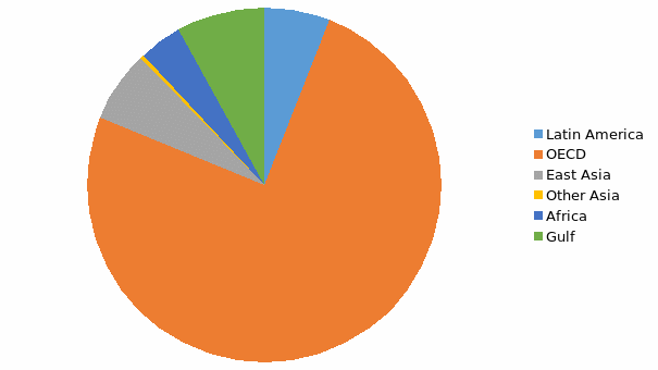
Based on the table above, the OECD region has the highest total GNP per capita. The region with the least GNP per capita is other Asia. The pie chart below shows the total GNP per capita for the six regions.

The data of the regions can also be analyzed based on the average GNP for the regions. The table below shows the summary for the average for the regions.
From the table, OECD the highest average GNP per capita. It is closely followed by Gulf region. The pie chart pie below shows the average GNP per capita per region.

Scatter plot of the male life expectancy and female life expectancy
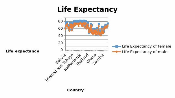
The diagram below shows a scatter diagram of life expectancy and female life expectancy for the 101 countries.

On average, the life expectancy of female (66.07) is greater than that of males (61.71). Female life expectancy ranges between 44 and 82 while male life expectancy ranges between 40 and 75. Further, it is evident that the life expectancy of both male and female for countries with higher GNP per capita is greater than countries with lower GNP per capita.
For instance, life expectancy in OECD countries is higher than life expectancy in countries in the Other Asia region. Also, within the regions, countries with higher GNP per capita such United Arab Emirates have higher life expectancy than countries with lower GNP per capita such as Egypt in the Gulf region.
Therefore, there is evidence of direct positive association between life expectancy and GNP per capita. However, it is not the only determinant of life expectancy. Good medical system in the economy also contributes a lot to higher life expectancy.
GNP per capita for African countries
The table below summarizes the GNP statistics for Africa.
From the table, Africa region has 31 countries with a total GNP per capita amounting $21,110. The average GNP of the 31 countries is $680.9677. Confidence interval testing will be used to test whether the average is statistically different from $300.
Hypothesis
Null hypothesis H0: mean = 300
Alternative hypothesis H1: mean ≠ 300
Test statistic – Use a two tailed T – test since the sample size is small
Level of confidence – 95%
Confidence interval = average value ± t tabulated * the standard error of the average
= 680.9677 ±2.042 * 81.72
= 680.9677 ± 166.7009
The confidence interval of the average of the African countries lies between $514.2668 and $847.6686. The interval implies that the average GNP per capita for all the countries in Africa is statically different from $300. Therefore we reject the null hypothesis at the 95% level of confidence and conclude that the average GNP per capita of countries in Africa is statistically different from $300.
Life expectancy of men and women
In general, it is always considered that the life expectancy of women is often higher than that of women across the world. For instance, in the data provided, the average life expectancy of women is 66.069 while that of men is 61.712. On the face of it, the life expectancy of women is higher than that of men.
However, statistically, the two values might be the same. Therefore, it is important to compute the statistical difference between the life expectancy of male and female. T– test can be used to test whether the means of the two life expectancies are statistically different. This would entail constructing confidence interval between the two means. Therefore, a confidence interval test will be carried out to find out if 66.069 is statistically different from 61.712.
Hypothesis
Null hypothesis H0: mean female = mean of the male
Alternative hypothesis H1: mean female ≠ mean of the male
Test statistic – Use a two tailed T – test since the sample size is small
Level of confidence – 95%
The difference in average value is 66.069 – 61.712 = 4.356
Confidence interval = average value ± t tabulated * the standard error of the average
= 66.069 ± 2.042 * 0.52272
= 66.069 ± 1.067
The confidence interval for the life expectancy of the female lies between 65.002 and 67.127. It is evident that the life expectancy of male (61.712) is not within that range. This implies that we reject the null hypothesis and conclude that the average life expectancy of females is statistically different from that of males at 95% level of significance.
Response and explanatory variables
In statistical analysis, it is important to separate between the response and explanatory variables. It is of much importance when carrying out regression analysis. Response variables, often known as predicted or dependent variable, represent the outcome of the study being carried out. It is the value that the regression analysis often aims to predict.
On the other hand, explanatory variable, often known as independent or predictor variable, explains the changes in the response variable. In most cases, the values are often determined outside the regression model, that is, In the relationship between GNP per capita and the percentage of adult literacy. The aim of the regression is to find out how the level of GNP per capita affects the percentage of adult literacy.
Therefore, the percentage of adult literacy is the response variable while GNP per capita is the explanatory variable. Therefore, regression analysis will be carried out of the percentage of the percentage of adult literacy level (Y) on GNP per capita (X).
Regression of percentage of adult literacy level (Y) on GNP per capita (X)
Regression analysis aims at finding the values of y intercept and values of various coefficients of the explanatory variable. The regression line line will take the form Y = a + bX. The theoretical expectation of the values will take the form a – take any value since it is an intercept while b should be positive (b > 0) since we expect a positive relationship between the percentage of adult literacy level and GNP per capita.
The results of the regression of adult literacy level (Y) on GNP per capita (X) is shown in the table below.
From the table, the regression line can be formulated as Y = 62.8232 + 0.0017X. The interpretation is that 62.82 is the percentage of adult literacy level that does not depend on GNP per capita. This can result from various factors such as free education offered by the state among others. The slope of the line that is, 0.0017 shows that a unit change in GNP per capita causes 0.0017changes in the percentage level of the level of literacy.
Plot of data points and the estimated regression line
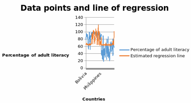
The diagram below shows a plot diagram of data points and estimated regression line.

The graph above captures regression line and data points for the percentage of adult literacy. From the graph, it is evident that the data points are erratic. However, the fitted regression line oscillates around the average value of the percentage of the literacy level which is 72.19%. Nevertheless, there are some points which are outliers that is, they are far away from the mean. Therefore, the regression line does not provide an adequate fit to the data.
Test of goodness of fit
Test of goodness of fit measures how well the estimated regression line explains the changes in the dependent variable that is how well the estimated equation fits the provided observations. There are various measures that can be used to test for the goodness of fit.
A commonly used measure is the coefficient of determination which is denoted as R2. R – squared value of 1 implies that the changes in the response variable are explained by the regression line. This is an indication of perfect fit. On the other hand, R – squared value of 0 indicates that the changes in the values of the response variable are not explained by the changes in the regression line. It indicates a poor fit.
The values of R – squared for the regression line of percentage level of literacy on GNP per capita is summarized in the table below.
From the table, the value of R – squared is 29.99% This implies that the regression line explains 29.99% change in the response variables. The value is very low and less than 50%. This implies that the regression line does not explain 71.11% of changes in the response variable.
The value of adjusted R – squared value is 29.27%. This implies that the regression line does not explain 71.73% of changes in the response variable. The values are quite low and it implies that the regression line does not fit the data point well.
Test of significance of the estimates
The table below shows the estimate values of the intercept and the slope of the graph. It also shows the t values and the standard errors that will be used for testing the significance of the variables.
To test for the significance of the intercept and the slope, t– test statistic will be used to estimate the values as shown in the computations below. The test will entail comparing the values of tabulated t and critical value of t.
Hypothesis
Null hypothesis H0: a = 0
(Implies that the value of the intercept is statistically not significant)
Alternative hypothesis H1: a ≠ 0
(Implies that the value of the intercept is statistically significant)
Test statistic – Use a two tailed T – test since the sample size is small
Level of confidence – 95%
The value of t – calculated is 24.6992
The value of t – tabulated at 95% level of confidence is 2.04
From the analysis above, t – calculated (24.6992) is greater than t – tabulated (2.04). This implies that you reject the null hypothesis at the 95% level of confidence and conclude that the slope is statistically significant. Therefore, we can conclude that the slope plays a statistically significant role in explaining the variation of percentage adult literacy level.
Similarly, test of significant can also be carried out on the slope of the regression line. Test of hypothesis will aim at explaining whether GNP per capita is a significant explanatory variable. The calculations are shown below,
Null hypothesis H0: a = 0
(Implies that the value of the slope is statistically not significant)
Alternative hypothesis H1: a ≠ 0
(Implies that the value of the slope is statistically significant)
Test statistic – Use a two tailed T – test since the sample size is small
Level of confidence – 95%
The value of t – calculated is 6.4792
The value of t – tabulated at 95% level of confidence is 2.04
From the analysis above, t – calculated (6.4792) is greater than t – tabulated (2.04). This implies that you reject the null hypothesis at the 95% level of confidence and conclude that the slope is statistically significant.
Therefore, we can conclude that the GNP per capita is plays statistically significant role in explaining the variation of percentage adult literacy level. Therefore, there is statistically significant relationship between the variables. The slope and the GNP per capita are significant determinants of the response variables.
Regression residuals
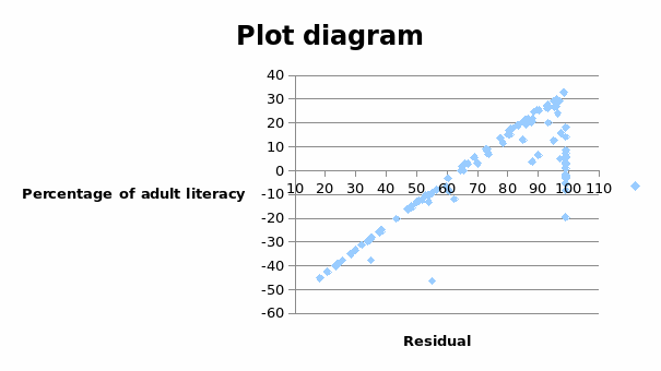
Residual denotes the difference between the response variable (Y) and the estimate variable. It is important to analyze the residuals since it shows the deviations from the estimated variable. The patterns displayed by the residual plots give more information about the data. Residual plots show the relationship between the response variables and the residuals. The response variable is on the X – axis while the residuals are plotted on the Y – axis. The graph below shows a plot diagram for the residuals.

The plot diagram above shows the relationship between the percentage adult literacy level and the residuals. The graph shows an upward trend. There is no randomness in the variables as expected. A random sample shows that the regression model fits the data. However, when the plot diagram takes certain shape, it implies that the regression line does not fit the data given.
In the case above, since the data is not random, it implies that the regression line does not fit the data. Further, there seem to be a linear relationship between the residuals and the response variable. The graph above could also be showing an indication of using other non linear relationship to estimate the relationship between percentage adult literacy level and GNP per capita.
Estimation
For New Zealand
The regression line is given as Y = 62.8232 + 0.0017X
GNP per capita for New Zealand = 12,780
The percentage of adult literacy = 62.8232 + 12,780*0.0017 = 84.5492%
For $100
The percentage of adult literacy = 62.8232 + 100*0.0017 = 62.9932%
For $20,000
The percentage of adult literacy = 62.8232 + 20,000*0.0017 = 96.8232%