Image Processing: Discrete Wavelet Transform Report (Assessment)

In arithmetical scrutiny and functional examination, a DWT (Discrete Wavelet transform) is any or every wavelet-transform under which the wavelet is discretely tested. As it is with other wavelet-transforms, a major advantage it possesses over Fourier transform in its sequential resolution: it also captures frequency together with position information -place in time.

Discrete Wavelet Transform

A DWT (discrete wavelet transform) of single-dimensional data is achieved when decomposition or the splitting of a signal is done in a set of 2 frequency bands (high and low). The low frequencies are once more decomposed into high and low frequencies. This procedure goes on on a random number of occasions which truly depends on the kind of application employed.

For the acquisition of the original signal an IDWT (Inverse Discrete Wavelet Transform) is needed, this can be obtained by employing the coefficients acquired from DWT. On the other hand, this re-enactment of the original signal from its DWT coefficients by use of IDWT can only be achieved if the filters for decomposition utilized, satisfy orthogonality the following condition.

|H(ω)|²+ |G(ω)|² = 1 (1)

The DWT conception for the one-dimensional signal can be broadened to 2-dimensional signals (images). This DWT2 (Two Dimensional Discrete Wavelet Transform2) is in fact recognized by working out the DWT transformation for the 2 dimensions independently.

Algorithm for adding watermark to the image using DWT2

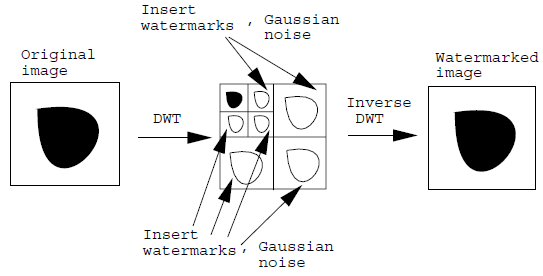
The algorithm for the addition of a watermark to the picture shown in [2] [3] is quite uncomplicated and easily comprehensible. The very first step to carry out is to decompose the picture into a number of bands by the use of Discrete Wavelet Transform. The coefficients of this acquired as a result, are supposed to be tailored in order to achieve the watermarked figure. Like for example, when we choose a Pseudo random-Gaussian noise for watermark, this noise is to be appended to the DWT2 coefficients. As per the algorithm presented in the paper, the choice of the DWT2 coefficients is of utmost significance because not every coefficient can be selected for this reason.

Coefficients of the superior frequency bands apart from those found at the lowest frequency band are preferred. The superior frequency bands’ coefficients are also shown as directional Horizontal, Vertical, and Diagonal (HVD) or comprehensive coefficients, whereas those found at the low-frequency band are referred to as estimated coefficients [1] [4]. For instance, if we let y(m,n) indicates the set of coefficients (that are not found at the low regularity band) and N(m,n) to be the Gaussian noise of 0 mean and harmony discrepancy, in that case, the new set of coefficients is acquired from the relation that follows.

ȳ(m,n) = y(m,n) + a × y(m,n)²× N(m,n) (2)

Here ‘α’ is the parameter’s control to fine-tune the intensity of watermarking in the picture. It should be also be taken into account that, there is a need to alter the approximation coefficients i.e. the ones matching to the low-frequency band. Now a 2D IDWT (Inverse Discrete Transform) is to be carried out by use of the new coefficient sets. This will be done with the addition of the Gaussian noise with the lowest frequency band coefficients not being changed. Hence the watermarked picture after re-enactment from IDWT2 is acquired.

Algorithm for detecting watermark to the image using DWT2

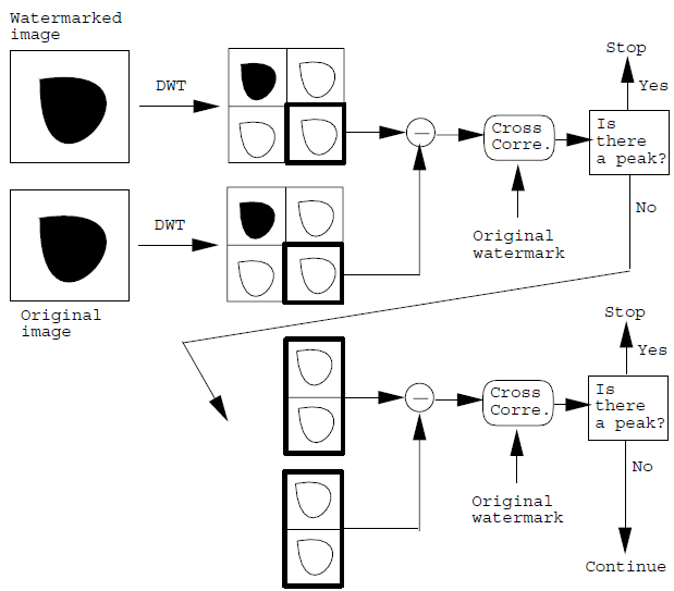
The recognition algorithm is found on the supposition that the original picture is known. By use of this, the original figure together with the watermarked figures are decomposed into 4 bands LL1 (Low Low band), LH1 (Low High band), HL1 (High Low band) and HH1 (High High band1). After that, the particular coefficients of the bands are evaluated and the dissimilarity in them is computed starting with the highest and the product, of which is convolved with the watermark. If the peak is established, this means that the digital watermark has been distinguished; or else the subsequent frequency bands in the pecking order are evaluated.

As in it is in the case of 4 bands, HH1 band of the original figure and HH1 band of the watermarked picture are evaluated and cross-linked with the watermark. If a peak isn’t seen, then HH1 and LH1 are evaluated. If the peak is seen, then this means the watermark has been distinguished. If not HL1 and LH1 are evaluated. Even as this is done, if the peak isn’t established the band of LL1 is additionally decomposed into 4 bands (HH2, HL2, LH2, and LL2), then the procedure goes on until a peak is distinguished or else the signature can’t be identified.

The following figures show the algorithm for adding up the watermark and identifying it [2].

Implement the algorithm of adding watermark for ‘lena.pgm’

The code for implementing the watermark addition to the image using DWT2 is placed below.

%% Watermarking

% Reading Input Image

I = imread(‘lena.pgm’);

% Setting the value of alpha

alpha = 0.03;

n = 2; % Decomposition Level

% Creating Low and High Pass Filters

[Lo_D,Hi_D,Lo_R,Hi_R] = wfilters(‘db1’);

% Decomposing in single level wavelet transform

[C,S]=wavedec2(I,n,Lo_D,Hi_D);

% Total approximate coefficients

total_app_coeff = 65536;

% Taking out only the detailed coefficients

det_coeff = C(total_app_coeff+1:end);

% Generating noise of 0 mean and 1 variance

N = randn(1,length(det_coeff));

% Adding Noise to the detailed coefficients using equation (4)

coeff_noise = det_coeff + ((det_coeff.^2).*N)*alpha;

%Creating new vector of coefficients for reconstruction of image

C_new = [C(1:total_app_coeff),coeff_noise];

% Reconstructing the image

I_new = uint8(waverec2(C_new,S,Lo_R,Hi_R));

% Displaying the results

figure(‘Name’,’Digital Image Watermarking’);

subplot 121;imshow(I);title(‘Original Image’);

subplot 122;imshow(I_new);title(‘Watermarked Image’);

The results thus obtained are as follows.

Discussion about the code

The outcome explained above, is achieved by use of a value of alpha=0.03 that can be augmented or reduced to manage the quantity of watermark in the figure. Image decomposition has been done on the original image in 2 levels by use of “wavedec2” MATLAB function [1]. Wavedec2 does decomposition on the picture into inputted amount of levels by use of an assortment of filters for decomposition purposes. A comprehensive list of obtainable filters can be established in [1], though I have used the haar filter also shown as db1-filter. After that the function produces a row vector ‘C’ having all coefficients of every band and a bookkeeping matrix ‘S’ having information on the dimensions of coefficients at every level[1] [4]. Coefficient vector C is again arranged in a way where it contains all the estimations coefficients at 1^st place.

Afterward the rest of the vector is packed with comprehensive/directional coefficients. The estimation coefficients are followed by flat feature coefficients, then perpendicular detail coefficients and finally slanting detail coefficients. Therefore since we do not require the estimated coefficients another vector having detailed coefficients only is produced which is then employed to put noise in, this is in accordance to the equation above (2) and the equation (4) in [2].

The latest set of coefficients acquired is joined with the estimated coefficients, which is then used for reconstructing the figure by use of MALTAB’S function IDW2, “waverec2”.

Implement the detecting algorithm (optional)

The code for the detection of watermark is presented below.

%% Q#3——-Detection

[C1,S1]=wavedec2(I_new,1,Lo_D,Hi_D);

% Diagonal detailed matrix i.e HH1 of Original Image

D1=detcoef2(‘d’,C,S,1);

% Diagonal detailed matrix i.e HH1 of Watermarked Image

D2=detcoef2(‘d’,C1,S1,1);

% HH1 of I_new minus HH1 of I

diff = D2-D1;

% Reshaping the difference matrix

diff = reshape(diff,1,size(diff,1)*size(diff,2));

% Correlation of difference with the watermark which is noise in our case

HH1_corr_HH1 = xcorr(diff,N);

% Plotting the correlation

% Here we can see that a peak is detected which means that the watermark

% has been detected.

figure(‘Name’,’Correlation’);

plot(HH1_corr_HH1);title(‘Differnce of HH1 and HH1 correlated with Noise’);

% Though the peak has already been detected and there is no need to check

% HH1 of original image with LH1 of watermarked image but its is good to do

% it again.

% Diagonal detailed matrix i.e HH1 of Original Image

D1=detcoef2(‘d’,C,S,1);

% Horizontal detailed matrix i.e LH1 of Watermarked Image

H2=detcoef2(‘h’,C1,S1,1);

% LH1 of I_new minus HH1 of I

diff = H2-D1;

% Reshaping the difference matrix

diff = reshape(diff,1,size(diff,1)*size(diff,2));

% Correlation of difference with the watermark which is noise in our case

HH1_corr_LH1 = xcorr(diff,N);

% Plotting the correlation

figure(‘Name’,’Correlation’);

plot(HH1_corr_LH1);title(‘Differnce of HH1 and LH1 correlated with Noise’);

Discussion and results

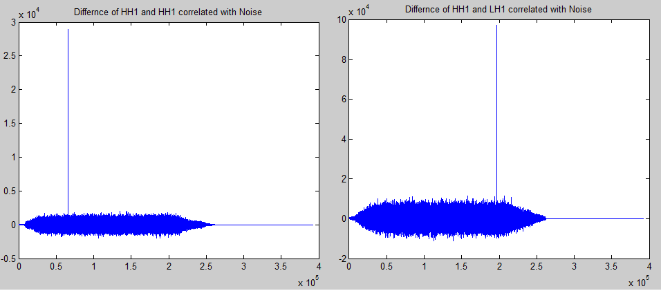
The code mentioned above used for detecting watermarks has been written to weigh against HH1 bands of original and watermarked figures equally. This is in addition to the evaluation of HH1 band and LH1 band of the original and water marked figure correspondingly. It has also been noted that, the peak is established in the 1^st attempt when evaluating HH1 bands of 2 figures, but to verify HH1 and LH1 bands of 2 images are once more compared and cross-correlated of the dissimilarity of 2 band’s coefficients. This is done when the Noise has been removed and a clear peak is achieved. The following are the results achieved.

Conclusion

Wavelet Transform is of late well-liked when it comes to examination, de-noising and compressing of signals and imagery. As shown in this paper the functionality employed to carry out singular and multilevel DWT (Discrete Wavelet Transforms), DWT or IDWT transform is employed to attain 4 dissimilar frequency figures. Watermarking is entrenched in elevated frequency picture by single value decomposition. This is different to traditional perspectives that presume watermarking is supposed to be embedded in low and mid frequency to acquire good robustness. Investigational estimation reveals that the projected algorithm can endure a variety of attacks that includes frequent geometric attacks.

References

MATLAB HELP.

Xiang Gen Xia, Charles G., ‘Wavelet transform based watermark for digital images’, OPTICS EXPRESS, Vol. 3, No. 12, 1998.

Multi-resolution Watermark Based on Wavelet Transform for Digital images By Vallabha VH Cranes Software International Limited. Web.

Digital Image Processing Using MATLAB Gonzalez, Woods, and Eddins, Prentice Hall © 2004.