Intelligent Agents for E-markets: Nash Equilibrium Essay

Introduction

Approximately 60 years ago Morgenstern and his counterpart von Neumann started the study of game theory. There is a mathematical result as an indication of equilibrium. This is in the sum game of two players. This model is where one agent’s gain is the loss of the other agent. This led to Dantzig’s linear programming system for optimization problems, as well as Yao’s principle for solving algorithmic lower bounds. Sometime in the last century, Nash proposed to explore the general multiple agent game-model, and where it was proven that mixed strategies exist called Nash-equilibrium point, one for each agent, such that no agent can benefit if it changes its strategy.

Nash equilibrium

Nash equilibrium is a name derived after John Forbes Nash who proposed it. It is a game theory, which is a solution concept of a game that involves two or more agents, where each agent is taken to know all the equilibrium strategies of the other agents, and no agent benefits by changing only his/ her strategy. If an agent has chosen a strategy and no agent has anything to gain if he/she alters some rules while the other agents do not change their ones, then the set of strategic decisions and the payoffs will create Nash equilibrium.

Bayes– Nash equilibrium is then a strategy aspect that states that no agent can get a higher expected utility if he/she departs from a strategy that is different from the agent’s beliefs about the dispensation of some cases from which other agents are excluded.

In Nash equilibrium, there is an assumption that an agent is using the strategy the other can do no better than using herself. It is not applicable in a negotiation setting. This is because it needs a utility function for both sides. It is, however, of interest to designers of automated agents. It avoids a need for secrecy by the programmer. There is a publicly known strategy for an agent, and the other agent designers cannot exploit the information by choosing a different strategy. The strategy should be public (should be known) to avoid inadvertent conflicts. This is helpful in the field of agreeing in the game theory. The players’ strategies are very important and hence there is a need for them to be accepted as they are played.

Pseudocode for the Nash equilibrium algorithm

These algorithms for Nash Equilibrium may be explained as follows:

1. Choose a set of strategies S where one can choose to search from the range [0; 1]. (Note: for the Large payment rule, a more reasonable search set is [¡:5; 5], as the rule provides incentives for agents to bid more and ask less than their true value for each bundle).
2. Select some s0 2 S in a random manner
3. Take a number n of valuation instances, based on the initial distributions of values & bid amounts.
4. Assuming that all agents other than ai follow strategy s0, compute the surplus ui over the n samples for agent ai for each of some set of strategies S0, where S0 µ [0; 1] is not necessarily a subset of S (see below).
5. Take the s¤ 2 S0 with the highest expected utility as an estimate of the ex-ante best response to s0.
6. Let s0 take on some new value between s0 and s¤, and repeat steps 3-5 until convergence is the set of agents.

   • Xi = is the group of activities which are assumed by player i, where yi is the number of available strategies for the player. The ai is a variable that takes on the value of an action aik for i, and a = (a1 an) to indicate levels of strategies, one for each agent. In addition, let a−i = (a1.. ai−1, ai+1,..an) denote a similar profile on the action relating to the participant i, so that (ai, a−i) creates a complete profile of strategies. We use the identical abbreviations in all the profiles possessing an ingredient for each player.

   An example:

   ui : X1 ×… × Xn → ℜ is a utility function for each agent i. It maps a profile of strategies to a price. Every participant i chooses a set strategy combinations which is available:

   Zi = . A mixed strategy for an agent shows the probability distribution used to choose the strategy used by the perticipant. We will sometimes use ai to denote the strategy in which zi(ai) = 1. The support of mixed strategies zi is the set of activities ai ∈ Ai given pi(ai) > 0. a = (a1,..am) is what we are going to utilize it to show a profile of trades that specify the size of the support of each agent.

   The first part of defining a strategy is assigning trades to each of the agents. We always choose to maximize the expected surplus of the agents. Let ¸ = (¸1; ¸2; :::; ¸TIj) denote a set of actions across all agents in T. We wish to find ¸r such that ¸r= arg max¸2r Xi2Ivi(¸) where, r, denotes the set of all actions across all agents. A play is considered feasible if for every positive allocation of a trade, there is also a negative allocation .

   The difficulty with the above calculation is that it is quite hard to solve exactly for a combinatorial exchange, because the problem is the same as solving maximum – weight set – packing. As noted, there are several algorithms for solving the exchange, and people use the method of solving for the maximum of the expected surplus by using certain commercial MIP solvers (Daskalakis, 2008). This is critical as we arrive at the designated activity and the equilibrium is as expected in the coming up with the solution. The importance are quite many and can be attained at any conclusion in the derivation. We have a game S = (N, A, u) where N represents the number of agents and A =A1 x … x An is an action set for the agents. All the action sets A_i is finite. Let Δ= Δ1 x … Δn represent the set of mixed actions for the agents.

   We can define gain functions as follows.

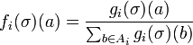
   For a mixed strategy σ∈Δ , it is possible to benefit for agent i on strategy α∈Ai be

   The gain function shows the benefit an agent gets by unilaterally changing his action. We can define g = (g1 … gn) where for σ ∈ Δ, σ ∈ Ai.

   We find that

   We now use g to show as follows. Let For α ∈ Ai.

   It is not hard to see that each f_i is a set in Δ_i. in addition, it’s simple to get that each f_i is a continuous function of σ, thus f is a continuous function. Now, Δ is the product of a final results of a compact convex set, thus it is necessary to admit that Δ is also compact and convex in such a case. The Brouwer non-variable theorem is to be utilized to f. Hence, f has fixed points in Δ, call them σ ^*.

   This is the proof that σ ^* is a Nash Equilibrium in G. It suffices to show that

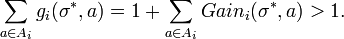
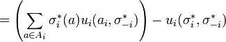
   This shows that the each agent gains no benefit by unilaterally changing his action, which is the necessary condition for being a Nash Equilibrium. We may assume that the gains are not all 0. Therefore,∃i , 1 ≤ i ≤ N, and α ∈ Ai such that Gain_i(σ ^* ,a) > 0. Note that

   Let . In addition, we may denote as the gain vector indexed by strategies in A_i. Since f(σ ^* ) = σ ^* we have that

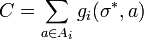
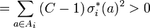
   Therefore, we find that

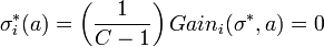
   Since C > 1 we get that σi is a positive scaling of the vector .

   Now we claim that .

   Given that Gain_i(σ ^* ,a) > 0, it agrees with the gain function. Assuming Gain_i(σ ^* ,a) = 0. Based on our earlier notes,

   This is equal to a zero hence the whole illustrations is zero.

   Therefore;

   The final inequality is next since σi not a vector. This is indicates opposing sentiments where all the positives have to be zero. We thus conclude that σ ^* is a Nash Equilibrium for G.

   This game has three Nash equilibriums with payoffs (2, 7), (7, 2), and (4 2/3, 4 2/3). The players may obtain higher payoffs if they could randomize over the joint actions space. For example, the following distribution of probabilities over strategy pairs is impossible if the players randomize independently, but feasible (Deng, 2005).

   The payoff is (5, 5). The point of correlated equilibria is that the players act in accordance with a randomization mechanism defined on their joint strategy space. Imagine a referee observing outcomes of a random process and announcing to each player what he has to do according to those out comes. The agents only know the probabilities over the joint strategies. Formally, we have the following model: Let G be an n-person game, and denote by S? 1 < i < n agent /’s the strategy space. S is the Cartesian product over the sets Si. Let u?: S ? R be the utility function for agent /. A correlated strategy n-tuple is a random variable from a finite probability space r into S. Such a correlated strategy n-tuple captures joint randomization. Define as the distribution of a correlated strategy n-tuple / the function that assigns to each n-tuple s of actions the number Prob f~l(s). The function / can be written as / = (fi,…, /?), and we set (fi, gi) = (fi,…, gi,…, fn). E denotes expectation. We can then define a correlated equilibrium: A correlated strategy n-tuple in G is a correlated equilibrium if and only if Eut(f) > Eui(f, gi) for all / and functions g? which are functions of f. Every convex combination of Nash Equilibria is a correlated equilibrium, but there might be correlated equilibria, which are outside the convex hull of Nash Equilibria (the one given).

   Utility function for agents

   Define a value vi for the minorant game and a value V2 for the majorant game:

   • vi = max min u i(s, t) and seSi teS2
   • v2 = min max u2(s, 0
   • teS2 seS

   We are able to see that, vi < v2. Von Neumann and Morgenstern claim that if there is a value v for T, it must be v < v < v2 (p. 106). For T1 describes player l’s most favorable situation and T2 describes player 2’s most favorable situation. So these two outcomes should constitute limits for what to expect for T. Von Neumann and Morgenstern want to continue without making any assumptions about “the players’ intellects”. There is an indication that the satisfactory theory is in existence when two extremes, T1 and T2 are easily accessible, strategies of player 1 ‘found out’ and strategies of player 2 ‘found out.’ This will lead to the introduction of the set strategies, which are defined, by the minorant game and a majorant game which have a direct relationship with the mixed algorithm.

   Conclusion

   Many thought the problem of finding a Nash equilibrium is complex. Many agents recently have proven that. It is not clear whether the 2-agent issue is to be indicated similarly as in the issue of PPAD-complete problems. Our work settles this issue and the open problem that has attracted Economists, Mathematicians, Operation Researchers, and most recently Computer Scientists. The result shows the richness of the PPAD-complete class introduced by Papadimitriou fifteen years ago. The Nash equilibrium has been indicated in this assignment and that all the dominant strategies being played by the agents will be at equilibrium where the respective agent plays as per the given specific strategy.

   References

   Daskalakis, K. (2008). The Complexity of Computing a Nash Equilibrium. New York: ProQuest.

   Deng, C. (2005). On Algorithms for Discrete and Approximate Brouwer. New York: Cengage Learning.

   Gul, F. (2000). The English with differentiated commodities. Journal of economics theory, 92, 66 – 95.