The purpose of the present laboratory work was to determine the nature of the relationships between the various variables describing the state of a gas using the ideal gas equation. Specifically, the variables were represented by temperature, volume, pressure, and mole number.
Background
The ideal gas equation [1] was formulated by Clapeyron in the nineteenth century; a universal equation describing the behavior of a theoretical gas that has the properties of an ideal gas. In particular, such properties include the assumed negligible size of the particles composing the gas, as a result of which no inelastic interaction is observed between them (LT, 2022). It follows that in a limited volume of an ideal gas, no inelastic collisions occur. Although this model is hypothetical, it can cautiously be applied to real gases at moderate temperatures and pressures.

The advantage of the ideal gas equation is that it is an empirical combination of several gas laws at once, establishing the relationship between several gas characteristics depending on which of the parameters have been chosen to remain unchanged. For example, Boyle’s law [2] establishes the relationship between the pressure and volume of a gas while keeping the temperature and mole number unchanged. It follows that an increase in gas volume leads to a natural decrease in pressure and vice versa. Gay-Lussac’s law [3] demonstrates that with constant volume and number of moles, the pressure linearly depends on the temperature: when one parameter increases, the second one also increases. Equation [4] shows Charles’s law, which indicates the relationship between the volume and temperature of a gas when the pressure and the number of moles are kept constant. This indicates that an increase in temperature leads to an increase in volume. Finally, Avogadro’s law [5] defines the relationship between the volume and the mole number of a gas, provided the temperature and pressure are unchanged: this is also a linear relationship. Each of these gas laws generalizes to the ideal gas equation and can be derived from this with proper manipulation
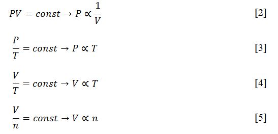
The relations between the variables defined above to describe the behavior of a gas can be explained in terms of the kinetic theory, the state of the particles entering the gas. The basic principles of this theory, in addition to understanding the atomic (or molecular) structure of gases, are the recognition of their continuous chaotic motion and the existence of absolutely elastic collisions between them (OS, 2022). In particular, in Boyle’s law, as the volume of the gas increases, the particles have more room to move and collide less often with the walls of the container, which reduces the pressure. In Gay-Lussac’s law, increasing temperature causes particles to communicate more thermal energy, which intensifies chaotic motion, and so the probability of collisions also increases, which increases pressure. Charles’s law is also explained: more active motion of the particles increases their divergence from each other, which causes the volume to increase. Finally, Avogadro’s law is explained by simply increasing the number of particles, which leads to occupying more volume.
Method
The methodological basis of this laboratory work was to perform a virtual experiment, the essence of which was to fix some variables unchanged and observe the behavior of others. The experiment was performed in a virtual environment, which saved resources and time on data collection. A total of four distributions were collected depending on which pair of variables were observed and which gas law was being evaluated. The data were recorded in an MS Excel spreadsheet, double-checked, and used to construct visualizations. Precisely, line charts were plotted for each distribution because each of the variables was quantitative, and continuity was implied because the thermodynamic parameters used were not discrete.
Data and Analysis
Table 1 shows the results of the direct measurements of volume, pressure, temperature, and mole number depending on which of the gas laws was evaluated. Each of the four variable distributions was visualized using MS Excel. Including a pair of volume and pressure variables to evaluate Boyle’s Law was further modified to determine the ratio of pressure to the inverse of volume.
Table 1. Results of direct measurements
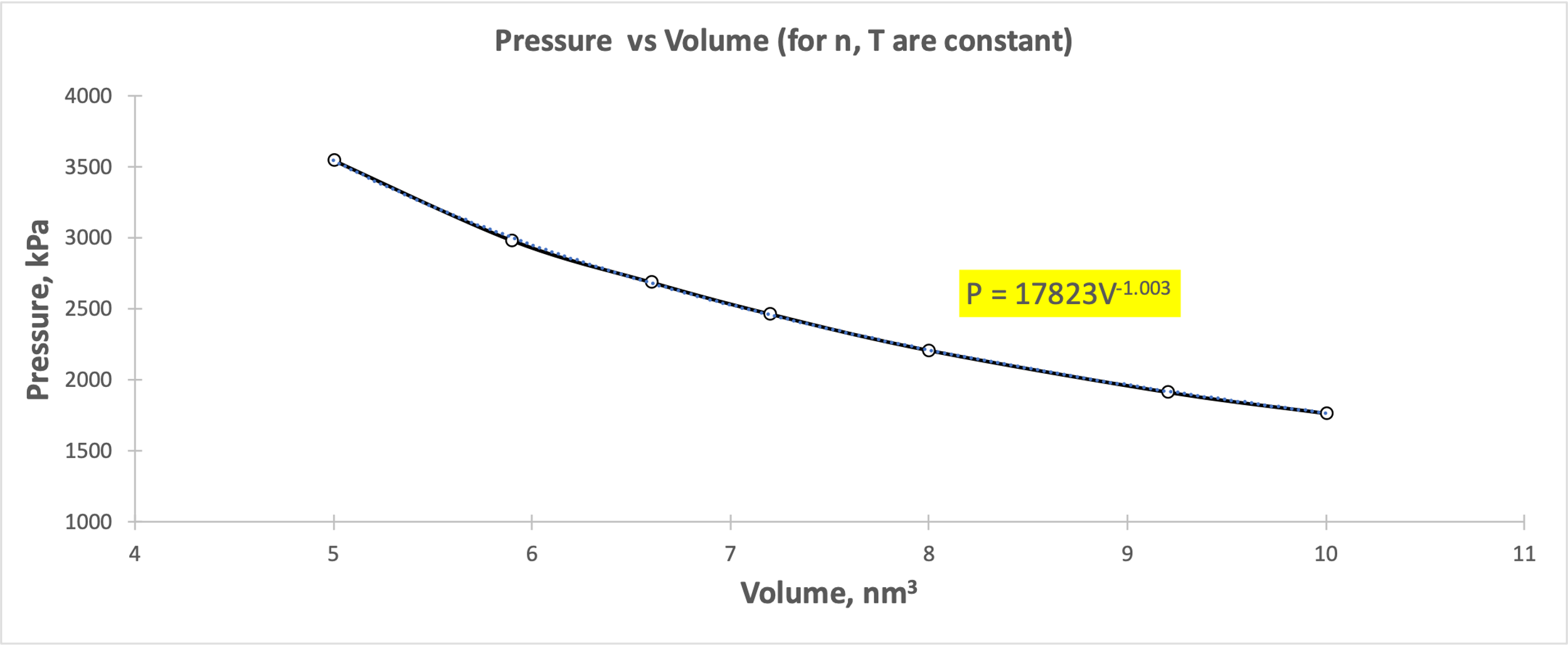
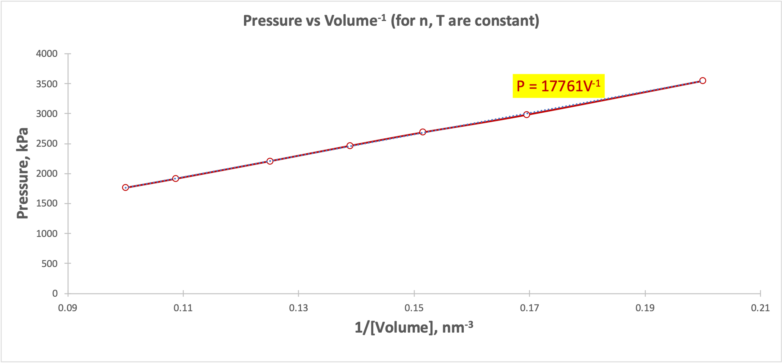
As can be seen from Figure 1, as the pressure increases, the volume decreases smoothly, and vice versa. There is no strict downward linear trend between the variables, but rather a partial hyperbolic form. From the point of view of kinetic theory, this behavior corresponds to the condition that the particles became distributed in a larger volume and decreased pressure systematically. Inverse volume as a predictor of pressure (Fig. 2) indicates a clear upward linear relationship, which confirms Boyle’s Law and Equation [2].
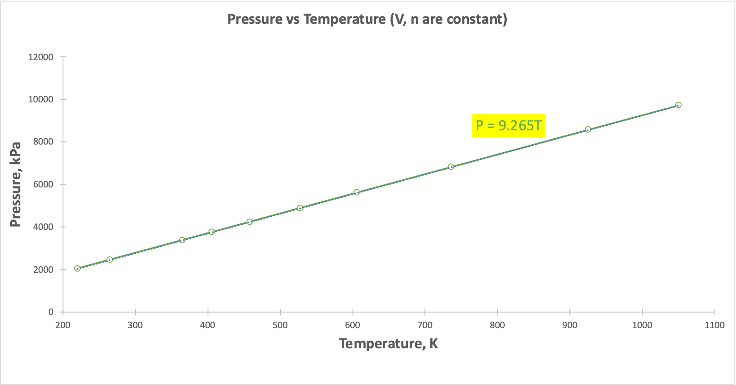
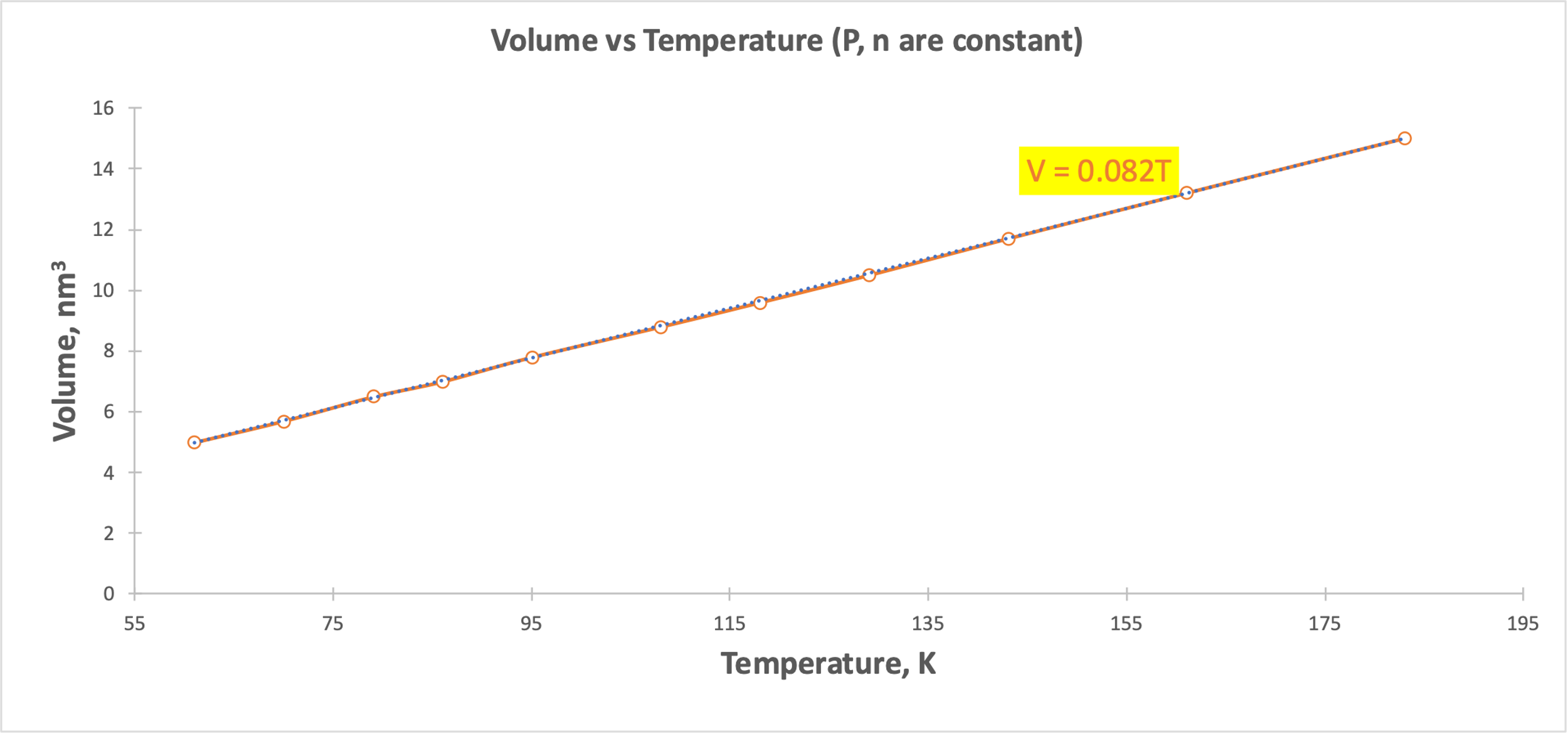
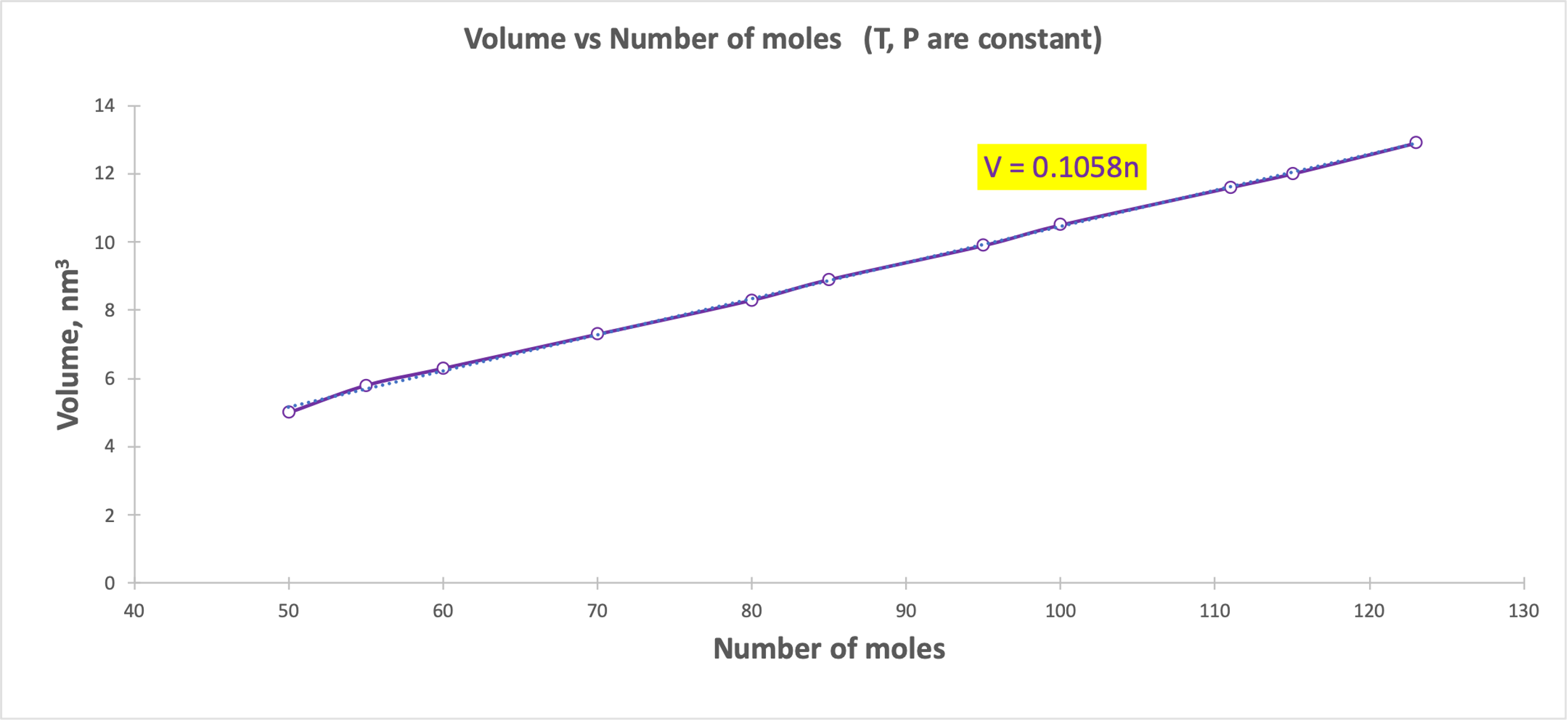
A linear relationship was shown for Gay-Lussac’s Law (Figure 3), Charles’ Law (Figure 4), and Avogadro’s Law (Figure 5). Figure 3 demonstrates that as the gas temperature increases, the pressure increases: the particles begin to oscillate with higher velocity, which leads to an increased probability of elastic collisions and increases the pressure. Figure 4 shows that when the temperature increases, the volume also increases linearly: more active chaotic motion becomes the reason for increasing the spatial distribution of the particles. Finally, when the number of particles increased (Fig. 5), it also increased the volume they could occupy and remain energy efficient. However, there is some deviation from the linear trend in Figure 5, which may be due to measurement errors or incorrect recording of the results. Thus, each of the visualizations confirms the gas laws. Each of the five plots also shows regression equations that confirm the nature of the relationship between the variables.
Calculations
Input data were used to perform the simulation calculations. Specifically, the number of moles was chosen randomly as 500, the temperature was set to 30 °C (303.15 K), the pressure was 2500 kPa, and the volume was 0.5 m3, according to SI. The simulation showed that in this case the gas constant R was equal to 8.247. The calculation, which was done automatically, is shown in equation [6]. It is noteworthy that the true value of R is 8.314 J.K-1.mol-1, which creates an error of 0.8%. This error could be due to the awarding of forced values of each variable in a limited space, and thus the gas could be unstable.

Discussion
Overall, the study was successful in that it confirmed the theoretical facts about the relationship between the various gas characteristics. From this experiment, I was able to learn how related all variables are, and how manipulation of some certainly affects others. Problems that arose during the experiment included inaccurate data, which in some cases led to errors. For research, minor errors are not a problem if one understands their cause, which has been accomplished. In the future, more data should be collected for each distribution of variables in order to obtain more reliable results.
Conclusion
The present work has validated the gas laws with simulation examples and has shown the nature of the relationships between them. The main conclusion is the need to study gases comprehensively and not focus on just one characteristic, since in reality, they are all related by the ideal gas equation. This equation can be obtained by a combination of gas laws, namely by combining [2], [4], and [5]. Equality between the two parts of the equation is conditioned by the gas constant R, the introduction of which allows us to obtain the ideal gas equation.

References
LT. (2022). The ideal gas equation. Libre Texts Chemistry. Web.
OS. (2022). 13.4 Kinetic theory: Atomic and molecular explanation of pressure and temperature. OpenStax. Web.