Gasoline prices have a significant effect on the macroeconomic indicators. The prices of gas and other macroeconomic indicators are interlinked. This paper studies how these inter-linkages occur. During the 1970s and 1980s, it has been observed that gasoline prices have a severe effect on macroeconomic variables like output, employment, and inflation. This paper aims to test the influences changes in gasoline prices has on output, employment, and inflation.
The paper tests the effect of three macroeconomic indicators i.e. gross domestic product (GDP), consumer price index (CPI), and unemployment rate. Four independent variables that are chosen are gas price per barrel, money supply (M2), hourly wage earnings, and net private domestic investment. The paper will investigate the possible effects of the change of gasoline price on changes in GDP, CPI, and unemployment rate. Further, the paper will also try to shed some light into the reason for the change and through the channel, the change occurs. For this purpose, regression analysis of the three variables is considered due to the independent variables.
How does gas price change affect inflation? For this, we consider consumer price index (CPI) as an indicator of inflation. Figure 1 shows that with increase in gas prices, there is an increase in inflation and vice versa. Therefore, both follow a similar direction of change. A regression analysis done on the log of change in CPI to log of change in gas price and money supply (M2). The analysis gives a r-square value of 78% implying that the effect of change in gas prices and money supply have 78% probability of affecting CPI. The linear regression equation that is derived from the analysis is CPI = 0.69 + 0.39M2 +0.13(Gas Price).
Therefore, the analysis indicates that an increase in Gas prices will induce and increase in money supply, which will again increase CPI. Further, the positive intercepts of M2 and Gas price indicate that an increase in gas price will increase CPI and so would M2. The ANOVA results of the regression show that the results are statistically significant at 0.05 level of significance. As gas prices increases, in order to purchase the same amount of gasoline, Federal Reserve pumps in more money into the economy, thus, increasing M2. As more money is pumped in, there is a rise in the money supply in the economy, creating higher rates of inflation, which is indicated by a higher price level i.e. CPI.
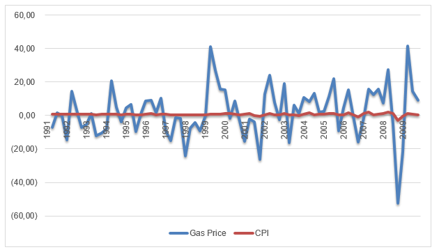
Figure 2 shows the change in unemployment rate is inversely proportional to changes in gasoline prices. As observed in 2008, when there was a sharp fall in gasoline prices, there was a marked increase in the unemployment rate.
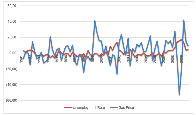
Table 2 gives the results of the regression analysis of log change in unemployment rate. The independent variables that are used in the analysis are log of CPI, output per hour, GDP, hourly wage, M2, gas price, and private domestic investment. The r-square value of the regression is 88%. The ANOVA results shows that the F-significance level is 0.00 implying that the analysis is significant at 0.05 level. The intercept that the regression analysis gives is negative i.e. -4.63. an increase in the gas price is found to be negatively related change in unemployment rate. CPI, M2, hourly wage, and private domestic investment are negatively related to unemployment rate. The linear equation that can be derived from the analysis is
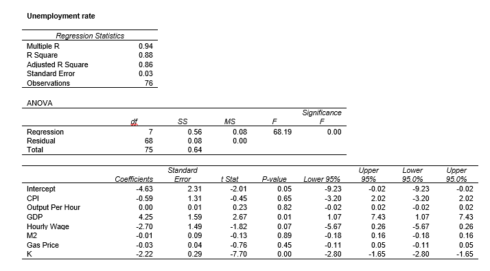
Unemployment rate = -4.63 -0.59CPI + 0.002 Output per hour + 4.25 GDP -2.7hourly wage – 0.01M2 – 0.03 gas price – 2.22K.
This suggests that with increase in gasoline prices, there is an increase in inflation, M2, nominal hourly wages. However, due to decrease in GDP and output per hour, there is an increase in unemployment rate. Thus, an increase in gasoline prices will reduce unemployment rate and vice versa.
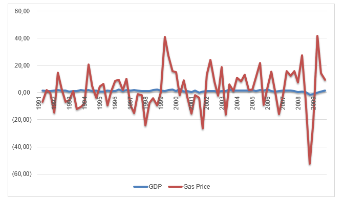
Next, the effect to gasoline price on GDP is considered. From Figure 3, it is apparent that there is some relation between changes in gas prices in the US with changes in GDP. Figure 1 shows, with increase in the change in gas prices, there is an increase in GDP and vice versa. The figure shows that the changes for gas prices and GDP follow the same trend and pattern. Therefore, the expected relation between gasoline prices change and change in GDP is positive.
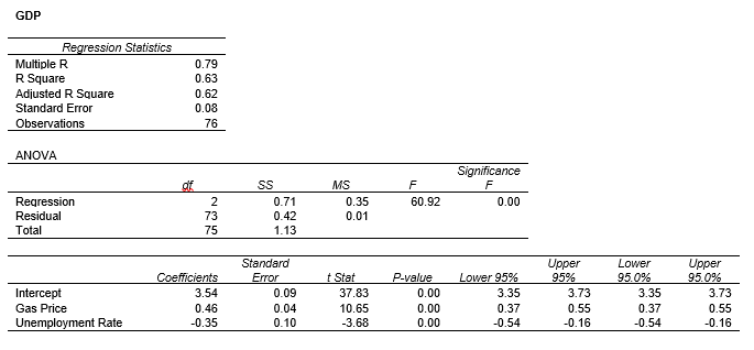
The regression analysis of GDP and unemployment rate and gas prices shows that the r-square is 63% (see Table 3). The ANOVA results show that the F-significance level is 0.00 i.e. less than the significant level at 0.05. the coefficients of the analysis show that GDP has a positive intercept. Further GDP is found to have a negative relation with GDP. The linear equation derived from the analysis is GDP = 3.54 + 0.46 Gas Prices – 0.35 Unemployment rate. This result is unexpected as figure 3 shows that there is a positive covariance of GDP and gas prices. The discrepancy may be explained through an increase in M2. As gasoline prices increase indicates an increase in inflation and thus an increase in M2 i.e. money supply in economy, there will be a rise in inflation. Higher inflation will lead to lower GDP.
Works Cited
Bureau of Labor Statistics. Labor Productivity Per Hour. 2010. Web.
Bureau of Economic Accounts. National Economic Accounts. 2010. Web.
Bureau of Labor Statistics. Average Hourly Earnings Of Production And Nonsupervisory Employees. 2010. Web.
—. Consumer Price Index. 2010. Web.
—. Unemployment Rate (based on a % of employment pool). 2010. Web.
Federal Reserve Statistical Release. Money Stock Measure. 2010. Web.
U.S. Energy Information Administration. Short-Term Energy Outlook – Real Petroleum Prices. 2010. Web.