Introduction
The analysis of data shows that it meets the assumptions of multiple logistic regression. The findings show that cholesterol level is a significant predictor of hypertension while age category, sex, and obesity are insignificant predictors. Hosmer-Lemeshow test shows that the model is statistically significant while scatter plots reveal that the apparent outliers do not make the model inadequate.
Assumptions
- The dependent variable ought to exist on a nominal scale (Field, 2012). The data have met this assumption because hypertension is a nominal scale with two categories.
- The independent variables can exist on a continuous scale, nominal scale, or ordinal scale (Forthofer, Lee, & Hernandez, 2007). The data have met this assumption for age category, sex, obesity, and hypertension are on nominal scale while cholesterol level and age are on a continuous scale. Cholesterol category exists on an ordinal scale for the scale represents increasing levels of cholesterol.
- Multicollinearity should not exist between two or more independent variables (Field, 2012). Age category and obese do not meet this assumption for they are collinear while other independent variables have met this assumption.
- The data points should not have influential cases (Forthofer, Lee, & Hernandez, 2007). In the data, scatter plots confirm that there are no statistically significant outliers.
Variables
Table 1. Variables and Level of Measurement
Simple Binary Logistic Regression
The First Model
The binary logistic regression results indicate that the odds of having hypertension among individuals with cholesterol levels of 200-299 and 300 or greater are 2.647 times (p = 0.04) and 13.714 times (p = 0.001) respectively higher than among individuals with under 200 cholesterol level.
The Second Model
The outcomes of the binary logistic regression indicate that the odds of hypertension increases by 1.012 times (p = 0.002) in every increase in the level of cholesterol among individuals.
Influence of the Level of Measurement
For the independent variable, the level of measurement determines its influence as a predictor variable. From the binary logistic analysis, nominal scale of cholesterol level has odds of 2.647 (p = 0.040) and 13.714 (p = 0.001) for 200-299 and 300 or above categories. In contrast, the ratio scale of cholesterol level gives an odds ratio of 1.012 (p = 0.002), which is lower than that of the nominal scale.
Since the level of measurement of the independent variable (cholesterol level) gives different odds ratio, it has changed my interpretation of odds ratio for I perceive it as a change of dependent variable for each unit change in the independent variable.
Multivariate Logistic Regression
Logistic Model
Table 2
Odds Ratios and the Significance of Each
- The odds ratio of hypertension among individuals with 200-299 cholesterol is 2.397 (p = 073) while that of individuals with 300 and above cholesterol level is 12.227 (p = 001).
- The odds ratio of hypertension among individuals with age category of 40 and above is 1.325 (p = 0.440) and the odds ratio of hypertension among women is 0.837 (p = 0.623).
- The addition of other variables has reduced the odds ratio of hypertension among individuals with 200-299 and 300 and above cholesterol levels from 2.647 and 13.714 to 2.397 and 12.325 respectively.
Hosmer-Lemeshow Test
The Chi-square statistic of Hosmer-Lemeshow test means that the logistic regression model fits the data, according to the assumption of goodness of fit, X(5) = 3.380, p = 0.642. A p-value that is less than the significance level (0.05) rejects the model for it does not fit the data while a p-value that is greater than the significance level (0.05) shows that the model fits the data (Hosmer & Lemeshow, 2004).
Logistic regression model
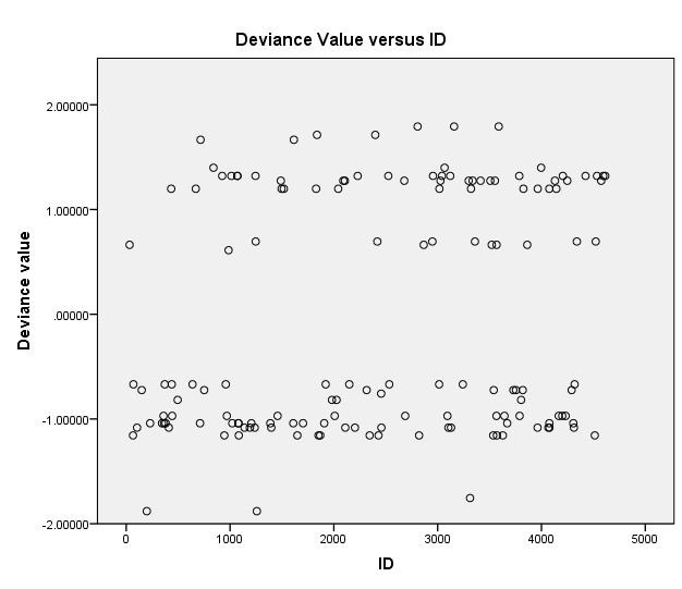
Scatter Plot of Deviance Residuals versus ID
The scatter plot (Figure 1) shows that there are outliers in the distribution of data points. In the evaluation of the logistic regression model, the presence of significant outliers implies that the model does not fit the data.

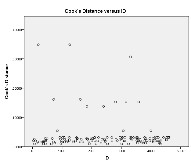
Scatter Plot of Cook’s Distance versus ID
Cook’s distance as shown in the scatter plot (Figure 2) depicts that there are influential cases in the data points. Specifically, there are ten influential cases, which have Cook’s distance of more than 0.1. The existence of the influential cases means that the model does not accurately fit the data, and thus, these cases require consideration to enhance the fit of the model.

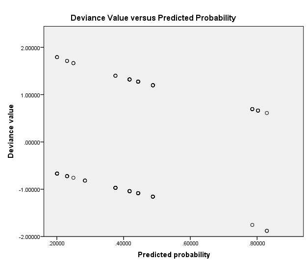
Scatter Plot of Deviance versus the Predicted Probabilities
In the scatter plot (Figure 3), the distribution of data points does not cause concern in the model for the apparent outliers in Figure 1 and Figure 2 do not have a significant impact on the model. Therefore, the scatter plot shows that the model is adequate in predicting the relationship between the dependent variable and predictors.

References
Hosmer, J., & Lemeshow, S. (2004). Applied logistic regression. Hoboken, NJ: John Wiley & Sons.
Field, A. (2012). Discovering statistics using IBM SPSS statistics. New York, NY: SAGE Publisher.
Forthofer, N., Lee, S., & Hernandez, M. (2007). Biostatistics: A guide to design, analysis, and discovery. Amsterdam, Netherlands: Elsevier Academic Press.