Pearson Correlation Coefficient and Linear Regression Dissertation

Calculating the Pearson Product-Moment Correlation Coefficient

The product-moment correlation coefficient allows for the calculation of two linearly dependent variables. In this case, the variables will be represented by x and y. The example to apply is a case of a pharmacy with an owner interested in knowing the time taken in the pharmacy (x) and money spent (y) by every tenth client in minutes and dollars, respectively. The assumption is that those who take a long time will spend more (positive correlation) and vice versa (Kenney & Keeping, 2011). To solve this puzzle, it is possible to compute the product-moment correlation coefficient denoted by r. The above case can be calculated as illustrated below.

Step 1

Step 2: Eliminate all the incomplete pairs. In doing this, observations with known values of x and y are included, even if the values are zero as illustrated in figure 2 below.

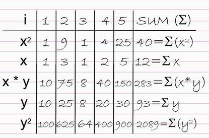
Step 3: Step three entails summarizing the resulting data into distinct values for computation by using the following signs.

n: Summation of pairs of data

Σ(x²): Summation of x values squared

Σx: Summation of the x values

Σ(x*y): Summation of each value of x which is multiplied by the y value that corresponds to the x values

Σy: Summation of the y values

Σ(y²): Summation of the y values squared

The above x and y values give the following figures when computed.

Step 4: Compute the ss_xy, ss_xx, and ss_yy with the above values as summarized below.

ss_xy=Σxy-(ΣxΣy÷n)=283-(12*93/5)=59.8

ss_xx=Σx²-(ΣxΣx÷n)=40-(12*12/5)=11.2

ss_yy=Σy²-(ΣyΣy÷n)=2089-(93*93/5)=359.2

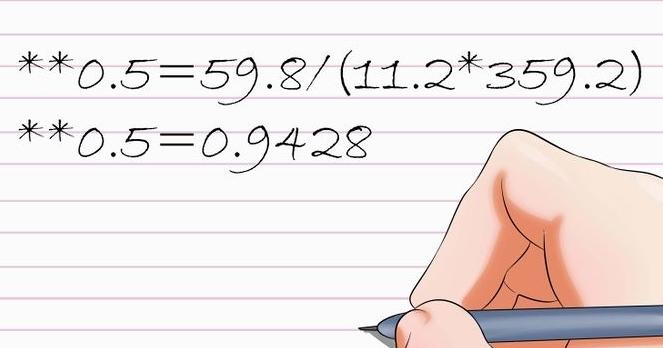
Step 5: The resulting values should then be inserted into the initial equation for the Pearson coefficient as illustrated below.

r=ss_xy/(ss_xx*ss_yy)**0.5=59.8/(11.2*359.2)**0.5=0.9428

Step 5: Interpreting the results

Option 1: When the value is close to 1, it indicates that there is a strong and positive correlation (Howell, 2016).

Option 2: When the value is very close to zero, it indicates no correlation.

Option 3: When the value is close to -1, it indicates that there is a strong and negative correlation.

In this case, since the value is 0.9428, which is very close to 1, there is a strong positive correlation between time and money spent in the pharmacy.

Calculating Simple Linear Regression

A simple linear regression explains the link between variables with the use of a straight line (Mugenda & Mugenda, 2013). For instance, consider data collected from a health center on different tests where each yield is associated with the temperature reaction as summarized in the figure below.

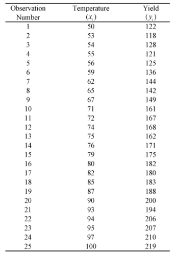
The above data can be entered in Microsoft Excel and a simple scatter plot may be derived as indicated below. The variables of yield and temperature values are represented by yi and xi respectively.

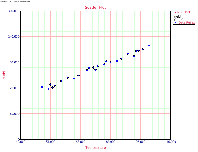
From the above scatter plot, there is no single line that can touch all the points. This is an indication that there is no linear relationship between yield and temperature for the tests. However, the scatter plot seems to suggest that a straight line might be drawn to touch specific points within the table. From a statistical perspective, the relationship between the x and y variables can be summarized in the equation below.

This means that the Y is assumed to be following a linear relation s summarized in the equation below.

The assumption in deriving a simple linear regression is that the values of Y are the summation of the E(Y) (mean value) and random error as summarized below.

References

Howell, D. (2016). Fundamental statistics for the behavioral sciences. New York, NY: Cengage Learning.

Kenney, J. F., & Keeping, E. S. (2011). Linear regression and correlation. Princeton, NJ: Van Nostrand.

Mugenda, C., & Mugenda, O. (2013). Applied statistics in research. Capetown, SA: CapeHouse Publishers.