Introduction
The purpose of this report was to investigate the simulation process of towing a bulbous bow ship on the water. An interesting feature of this ship is the bulbous edge located under the bow of the ship at the front of the model (Chakraborty, 2021). A scale model of this ship was used for the test, launched in a large water basin set up in the classroom. During the experiment, the vessel was placed in the water and experienced a load forcing it to move in one direction. The parameters of this motion were recorded, which included measuring the velocity at points in time, as well as studying the resistance characteristics of the ship. In the present work, these data were used to calculate integral and differential functions. Dependencies between the variables were also studied. Therefore, this report is a mathematical description of this process in terms of numbers, which can no longer be used in the simulation but in the real process.
Experimental Procedure
In this experiment, the model was placed in a large pool set up in the classroom and filled with water. During the movement of the vessel, water velocities were recorded automatically over time, and the data was recorded in a table. These data were transferred to Excel for further analysis. The first stage of this analysis was to process for ambiguity, namely, to cut off the end values of the function to minimize the error. Dependency plots were plotted in Excel, and large calculations of the desired values were performed. However, most of the calculations of the integral and differential functions in this work are manual and are shown in the following sections. Methodologically, this report was intended to answer the following questions:
- Is the dependence of velocity on time linear?
- What is the correlation effect between velocity and the R/V variable?
- What is the nature of the relationship between velocity and the R/V variable?
- What is the signal-to-noise ratio, or SNR for short, for velocity data?
Results and Discussion
Scatter Plot
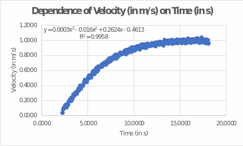
To work with the velocity and time data, a second test was chosen to represent the most informative data. For this purpose, the results were lightly processed, namely the left and right ends, where the velocity was initially zero and went down after reaching the peak values were removed. The figure below shows the scatter plot, which was the final representation of the data. It can be seen that the velocity as a function of time is not a linear function but increases slowly during the first ten seconds, after which it reaches virtually unchanging values. In such cases, the function is said to have reached a horizontal plateau (Ledwith, 2019).

For this figure, the information about the regression analysis is noteworthy. Excel is able to automatically select the best fit line for the data and show its equation, which is what is done in the figure. “Best” this fit between the set of points and the regression line is called because it covers the most significant amount of velocity variance (Chen, 2022). In this case, R2 determines the coverage to 99.58 percent of the variance, which is excellent.
Differentiation
The function shown in the figure determines the velocity behavior for the ship model:
For example, at time t = 5 sec., the function can be used to calculate the velocity of the ship:
However, this function can also be used to obtain a mathematical expression for acceleration by differentiation (Krista, 2021):
Accordingly, the acceleration function changes according to the parabolic law.
Integration
The original velocity function can also be used to calculate the mathematical expression of the path as a function of time. To do this, the dependence must be integrated, with time as the boundary of the defined integral. Ideally, one should use the time bounds shown in the figure above. However, with a certain margin of error, it is acceptable to extend these bounds to the left side up to time t = 0. Then:
The constant C is omitted if the integral has been determined. Then it does not need to be taken into account when substituting the time values:
It is correct to say, then, that in about eighteen seconds of testing, the ship managed to travel about 11.07 meters. In general, this is also true for the other four tests, in which the velocity function had a similar form, and the time frame was the same. That is, we can cautiously say that during each of the tests, the ship model traveled about 11.07 meters. Any deviations from this value for the other tests may be due to measurement errors and uncertainties (Schober and Vetter, 2018).
Regression
In the second part of the paper, resistance and velocity values were measured for the moving model in five trials. The data from these measurements are shown in the table below, which also includes the results of the automatic calculations for the regression analysis:
From this table the values of the regression coefficient can be calculated by the following formula:
And for specific data:
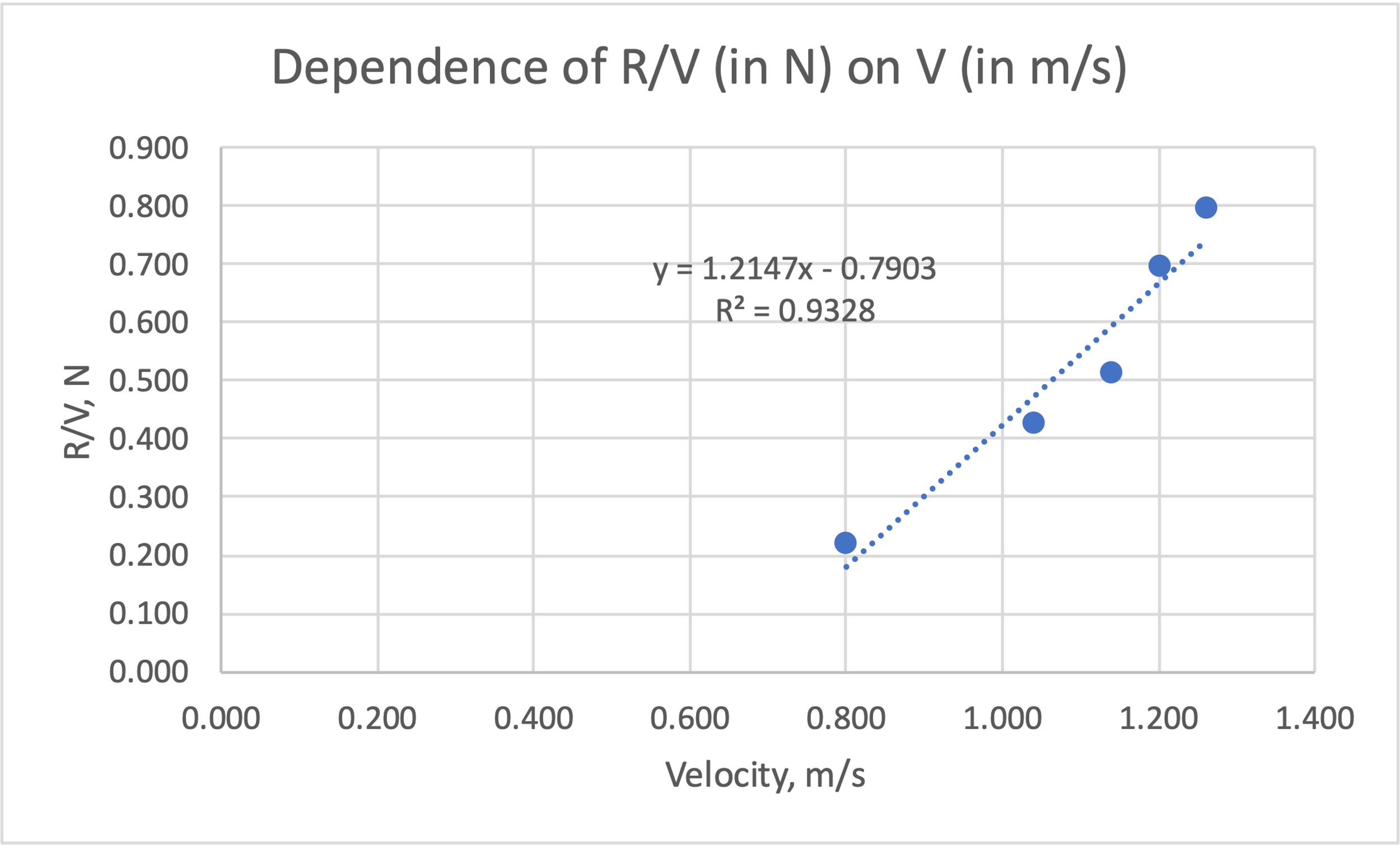
This indicates that there is a positive strong correlation between V and R/V, that is, they tend to rise or fall at the same time. At the same time, the coefficient R2:
It follows that the regression model can cover up to 93.3 percent of the variance in R/V. The regression equation is as follows:
And the coefficients a (gradient) and b (y-intercept) can be calculated by the following formulas:

Then the overall regression equation will be:
It follows that with increasing velocity there is an increase in R/V. And at V = 0, according to the regression equation, R/V should be negative. However, in reality, in the absence of velocity (V = 0), R/V should also be zero since there was no resistance. This deviation can again be explained by statistical error. The results obtained can be compared with the automatic Excel calculation:

That is, one can see that the manually calculated values correspond perfectly to the Excel calculations.
Signal-to-Noise Ratio (SNR)
The data from the fifteen points closest to the highest velocity from Appendix A can be used to calculate the SNR. The data that was used is shown below:
Formula for calculating SNR:
To do this, it was first necessary to find the arithmetic mean of the velocity values, this was calculated automatically using Excel:
At the same time, it was necessary to find the standard deviation for SNR:
Accordingly, the SNR value:
This means that the mean value is 45.32 times the standard deviation. In the context of SNR, this indicates an extremely good signal for data transmission. In telecommunications technology, the SNR value corresponds to a measure of signal accuracy, that is, how easily a signal can be separated from extraneous noise (Scaife and Smith, 2018). Since the SNR value obtained is quite high, it follows that the signal was reliable and accurate, the impact of third-party noise is minimal.
Practice Case Solution
In order to practice the mathematical skills, a practical calculation needs to be done. For this purpose, a time-dependent path function was proposed:
The function can be used to calculate the value of the path at a particular point in time, for example, t = 15:
In addition, the function can be differentiated to obtain an expression for the velocity:
After six seconds, the velocity is equal to:
And the time when the velocity was zero is defined as follows:
But time cannot be negative, so the velocity is zero when t = 1.884 seconds. We can also obtain an expression for the acceleration:
And four seconds later:
The acceleration was zero when:
The distance function could also be used to calculate the total distance traveled by the ship after ten seconds:
Conclusion
A water pool experiment was used to study the aerodynamic performance of a bulbous bow model ship towing. The report shows the mathematical calculations to determine the key values in this test. It was found that the velocity depends on time nonlinearly and is well described as a polynomial function. The results of a high positive correlation between V and R/V were also noted. Key conclusions of the study include the following:
- The equation of velocity as a function of time:

- Correlation coefficient:

Reference List
Chakraborty, S. (2021) What’s the importance of bulbous bow of ships? Web.
Chen, J. (2022) Line of best fit: definition, how it works, and calculation. Web.
Krista (2021) Position functions, and velocity, and acceleration. Web.
Ledwith, J. (2019) Exponential function and decay. Web.
Scaife, A.A. and Smith, D. (2018) ‘A signal-to-noise paradox in climate science’, Climate and Atmospheric Science, 1(1), pp. 1-8.
Schober, P. and Vetter, T.R. (2018) ‘Repeated measures designs and analysis of longitudinal data: if at first you do not succeed—try, try again’, Anesthesia and Analgesia, 127(2), pp. 569-575.
Velocity and Time Values (n = 532)

Values of Velocities and Resistances (n = 5)
