Simple Damped Harmonic Motion Determination Using an ‘Eyeball’ Analysis Report

Abstract

The motion of a freely swinging pendulum is believed to be a Simple Damped Harmonic Motion (SDHM), and as such it decays with time until it comes to rest (Papoulis 526). The objective of this experiment was to determine this motion using an ‘eyeball’ analysis. In this experiment, concurrent results of the ‘eyeball’ and the graphical analysis were taken for a swinging Styrofoam ball. The graphical analysis was used to confirm the ‘eyeball’ analysis. Prior to this twin experiments, the value of gravity g was determined using a pendulum bob (tennis balls) to enhance precision in subsequent calculations.

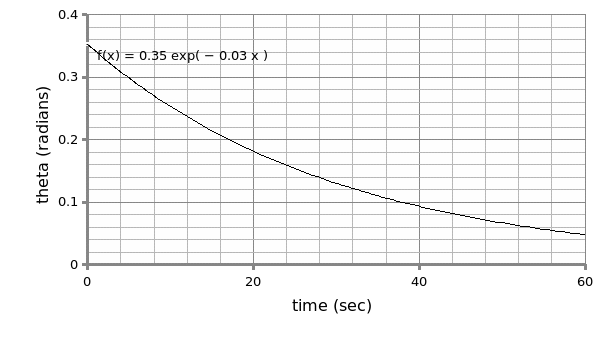
From the experimental results, the value of g was found to be 9.97m/s² as opposed to its theoretical value of 9.81m/s². This translated to an error of 1.63% thanks to external influence of forces within the earth which tend vary the gravitational acceleration form place to place. The calculated value was used to obtain the quality of the wave (448). This indicates that the wave will have to undergo 448 cycles before it decays. With regards to the sin fits of the motion, the ‘eyeball’ gave θ (t) =0.3℮ (-t/25) sin (3.77t+ Ø) while the graphical (computerized) fit gave θ (t) =-0.2927℮ (-t/26.56) sin (-3.758t+ Ø). The twin experiments gave almost analogous results were it not for the experimental errors. In future experiments, this experiment should be done in a laboratory free of wind motion to minimize errors that might have brought about the observed deviations.

Experimental Objective

The objective of this experiment is to investigate the motion of a swinging pendulum using an eyeball.

Procedure

In this experiment, two sets of experiments were set. In the first setup, the objective was to obtain a correlation between the periods, T, and the length, L, of a swinging pendulum. A tennis ball with a known diameter was set to oscillate 20 times about its center (at a small amplitude of 0.1 radians) while maintaining the length of the pendulum. L was varied six times momentarily while maintaining the amplitude. The periods and their respective lengths were recorded for analysis. Alongside this setup, one set of pendulum was used to draw the relationship between the amplitude and the period by varying the amplitude 5 times (between 5⁰ and 25⁰)

In the second setup, using a Styrofoam ball of a known diameter, the aim was to investigate damped harmonic motion (DHM). The ball was set to oscillate about its central position to decay to about 20% its amplitude. Using a sonar detector, a relationship between the amplitude and the time was obtained as the graph was being drawn concurrently.

Results

The results obtained were summarized as shown below:

For the first setup the relationship between T^2 and the length L gave a linear relationship with a gradient of 3.96 which is equivalent to a gravity of 9.97m/s^2. This differs slightly with the actual value of value (9.81 m/s^2) by 1.63%.

For the second setup, the results obtained for the constants for both eyeball and the graphical analysis almost coincided. The eyeball sin fit obtained was: θ (t) =0.3℮ (-t/25) sin (3.77t+ Ø). The graphical analysis fit obtained for the same motion was: θ (t) =-0.2927℮ (-t/26.56) sin (-3.758t+ Ø). The discrepancies in these constants are summarized as below:

The quality ‘factor’ obtained for the wave was 348 and the damping constant b obtained was 0.0003kg/s.

Data analysis

The table of the first setup is shown as below:

From the data above the graph of time^2 against length illustrate a linear relation as shown below:

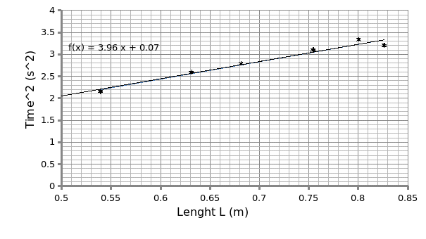
From the graph above, the relationship between periodic time (T) and the length of the pendulum is connected by the formula below.

• T = 2∏ [(L+D/2)/g]^0.5

Squaring on either side you obtain:

• T^2 = 4∏^2 (L+D/2)/g

On simplifying the equation you obtain the equation below:

• T^2 = (4∏^2)/g* L + 4∏^2D/2g

Since the graph of T^2 against L is a straight line, then the relationship assumes a linear relation and thus;

The slope (S) = (4∏^2)/g

Therefore,

g = (4∏^2)/ S

= (4*3.142^2)/ 3.96

= 9.969297375

≈9.97 m/s²

The experimental value of gravity (9.97 ms^-2) is almost equal to the theoretical value (9.81ms^-2). The discrepancy in this value is about 1.63%.

As per the graphical analysis of the eyeball, the table below was obtained.

θ= (Rs- Ro)/ L

L is the length of the pendulum Ξ 0.6855 m.

Therefore, θ= (0.600- 0.358)/ 0.6855

= 0.3530 rads.

The eyeball angular frequency w^I is give by the formula;

• w^I = 2∏/ T = 2∏f

From the graphical analysis, the pendulum is making 30 oscillations in 50 seconds therefore; the frequency f of the pendulum will be given by:

• f = 30/50 =0.6 Hz

Thus, w^I = 2*3.142* 0.6

= 3.77 radians/ second.

From the decaying exponential function F (t) =A℮^ (-t/ז) the following deduction can be made to obtain the decaying time ז: since F (t) =A℮^ (-t/ז) Ξ the function F (t) = 0.3℮^ -0.04t then;

-t/ז = -0.04t

Hence, ז = 1/0.04 = 25 seconds

The quality factor Q is obtained from the formula; Q =w_oז

But, w_o= g/ (L +d/2)

Hence, w_o= 9.97/ (0.6855 + 0.061/2) = 13.92

Therefore, Q = 13.92* 25

= 348

The dumping constant b is obtained from the formula: b= 2m/ז

Hence, given the mass of the Styrofoam as 0.00762 kilograms and the decaying time ז as 25 seconds; then:

b= 0.00762/25

= 0.0003048

≈ 0.0003 kgs/ sec

On fitting these parameters on a sine curve, θ (t) =θo ℮ (-t/ז) sin (w^I t +Ø), the below formula is obtained:

• θ (t) =0.3℮(-t/25) sin (3.77t+ Ø)

On comparing the eyeball sin fit parameters to the graphical analysis sin fit, the summary below is observed:

Discussion

The preliminary objective of this experiment was to first of all to ascertain the relationship between the periodic time and the length of the pendulum. This is believed to be related by the formula T^2= 4∏L/g (Papoulis 528). The aim was to confirm the value of gravity g which theoretically has a value of 9.81m/s² vital in determining the precision of the results. From the plot, the value of g was found to be slightly bigger (9.97ms^-2) which translates to an error of 1.63%. This can be attributed to natural forces within the earth which tend to vary the gravity. To enhance the precision in the subsequent calculations the calculated value is used. Consequently, using the same, the quality factor obtained was 348. The quality factor determines the rate of damping. In this case, the wave will make 348 cycles before it decays.

The sin fits for both the eyeball and the graphical analysis almost gave analogous results were it not for experimental error. The degree of deviations were2.49%, 5.87% and 5.30% for θo, ז and w^I respectively. As per the ‘eyeball’ sin fit, θ (t) =0.3℮ (-t/25) sin (3.77t+ Ø), the decaying time was 25 seconds. This indicates that the wave will take 25 seconds to decay to 0.368 of its original amplitude. With regards to the deviations in the values of the constants, precautions should be placed such that the experiment is performed in a calm environment devoid of wind motion to increase precision.

Conclusion

Generally the main objective of this experiment was met were it not for the slight deviations in the experimental design. This is so because the errors were minimal with regards to both sin fits.

Works Cited

Papoulis, Athanasios. “Motion of a Harmonically Bound Particle.” New York: McGraw-Hill, 1984. Print.