Soil erosion models (SEMs) are useful to understand the impact of agricultural practices, land use changes, reservoir sedimentation and evolution of the landscape (Wainwright et al. 2009a). In the past, soil erosion modelling developed in two directions (Lilly et al. 2009). One of the development frameworks concerns designing an empirically based erosion equation, such as Universal Soil Loss Equation (Sander et al. 2014). The other one is the development of process-based erosion models (PBEMs), assisted by computer simulation modelling (Müller et al. n.d.). In recent years, the advanced development of erosion modelling has been focused on understanding and representing the uncertainty associated with spatial modelling. With the assistance of geographic information system (GIS), erosion modellers are willing to predict erosion patterns and sediment traces (Nearing & Hairsine 2011).
The Difficulties and Limitations of PBEMs
In general, an appropriately constructed model should have the ability to predict long-term effects (results) based on short-term records (Nearing & Hairsine 2011). However, these records may not include extreme events such as 100-year return flood events, which can have a major impact on soil erosion. In such cases, it is most likely that the impact of extreme events will be underestimated. Other than this problem, the major difficulty in erosion modelling is data collection (Nearing & Hairsine 2011).
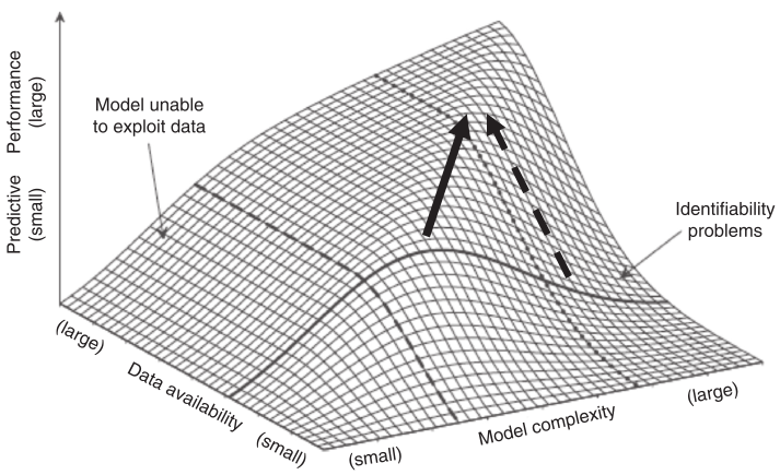
The limitations of PBEMs can then be distinguished into three types. First, it is hard to replicate all the natural variability in soil loss rates. Second, in extreme events and vulnerable conditions, it is hard to simulate the problems by using short-term data records. Third, it is hard to measure and quantify an extreme spatial variability of erosion on the landscape correctly (Nearing & Hairsine 2011). The quality of data is also a problem when GIS is required. For instance, a high resolution base map (normally a 1 km raster map) is the first step in processing a GIS-based analysis. However, this kind of maps requires a high level of power to gain access, and not all the countries are able to produce the map. Panagos et al. (2015) showed that this requirement restrains the accuracy of the final result of soil erosivity (also known as R-factor). The phenomenon of soil erosivity is typically defined as “the local rainfall’s ability to cause erosion” (Mercury study report to Congress, 2012, p. B-43). The balance between data availability and model complexity is also a problem faced while constructing models. In Figure 1, the solid arrow demonstrates the progressive development of soil erosion modelling, where extra complexity is reinforced by new data. The direction, in which the dashed arrow points, represents the scenario where new data is used with higher precision to constrain existing models (Nearing & Hairsine 2011).

Therefore, it is necessary to briefly evaluate the accuracy of Model of Assessing Hillslope-Landscape Erosion, Runoff and Nutrients (MAHLERAN) as a newly developed PBEM with limited literatures.
Aim and Objectives of the Project
The aim of the project is first to give a brief introduction of MAHLERAN, and, second, to test the performance of the model under different settings by controlling variables.
- Identifying the impact of flow-routing solution methods on end topography, flow velocity and discharge;
- Identifying the impact of updating topography on end topography, flow velocity and discharge;
- Identifying the impact of the number of iterations between topography updates on end topography, flow velocity and discharge;
- Identifying the impact of time steps on end topography, flow velocity and discharge.
Methodology
Model Description
Müller and others (n.d.) describe MAHLERAN as an erosion model, which simulates overland flow and sediment detachment, transport and deposition, based upon particle-travel distance for individual rainstorms. Unlike pure empirical models and equations, MAHLERAN is built on numerical methods with 50-years experimental data. As a PBEM, MAHLERAN implants an SE process, where interrill flow on hillslopes is controlled by rolling or sliding along surfaces, or through short steps, which are similar to the bedload movement. In order to apply this model, the following parameterizations are required: a specific site, spatial estimates of infiltration, flow roughness, vegetation, and particle size characteristics (Wainwright et al. 2009b).

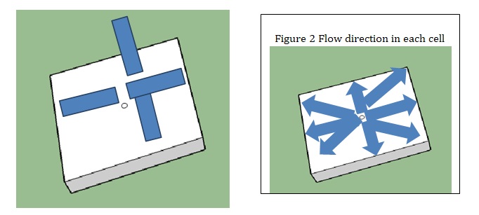
According to the MAHLERAN manual (Wainwright et al. n.d.), overland flow (assumed to be kinematic wave) velocity is calculated by the combination of 2D shallow water equations and the Darcy-Weisbach flow equation. Theoretically, the flow can run in four directions (as shown in Figure 2). But, in the case in point, the flow that is assumed to be running in the direction of the steepest descent is calculated. The flow routine is decided by the probability of how raindrops and sediments (soil) behave. Smith-Parlange infiltration model is applied to overcome the limitation of field data (Wainwright et al. 2009c). Particle sizes are catalogued into six classes. They are assumed to be transported through a splash, flow (concentrated/un-concentrated), or in a suspension. There are three ways for the detachment to occur: a) when there is no overland flow, raindrop detachment is the only way; b) when it is un-concentrated flow, surface layer effects are attributed to the modified raindrop detachment; c) when it is turbulent flow, concentrated erosion occurs. The deposition of sediment is modelled, using a transport-distance approach as described by an exponential distribution function (Wainwright et al. n.d.).

Advantages and Limitations of MAHLERAN
ArcGIS user friendly
MAHLERAN also generates the asc. File, which can be directly applied into ArcGIS. It allows researchers to study the sensitivity of the model by changing input codes (Dynamics of Runoff And Erosion Modelling (DRAEM) n. d.).
Improved accuracy
Since MAHLERAN considers not only empirical data but also numerical reasoning, it tends to be more accurate on predicting flow routine, unlike other empirical methods since the data can be disproved under certain conditions or limited on certain conditions, although obtaining natural rainfall data is important on studying climate differences (Meyer 1994). The application of MAHLERAN can help researchers identify the most important factors to the overall erosion process (‘Scales and erosion’ 2013).
Study of plantation
By uploading cropping distribution to the model, researchers can check the influence of the cropping distribution, hence, deciding the plantation method in interesting areas (What are the benefits of erosion and sediment control?, 2009).
More functioning
As it is introduced in 2.1, MAHLERAN can be used in interrill processes. It means that single processes of detachment and transport on interrill areas can be analysed. This is important because the results from models that can only predict the sediment yield from interrill areas can be experimentally determined (Nearing et al. 1994).
Limitations
Transition of the flow
As it has been mentioned above, in the model, the runoff flows through the centre of each cell and diagonally. This setting, hence, has simplified the behaviour of running water. It also miscalculates the amount of concentrated erosion that happens in one storm event (Wainwright et al. 2009c).

Limited literature and evidence
According to Wainwright et al. (2009c), MAHLERAN applies Hassan’s research on the relationship of transport distances and virtual velocities, which was obtained from a range of datasets in the channels, to hillslope condition.
No feedback on erosion and surface topography
Due to the computing efficiency and numerical stability, the model does not provide feedbacks on this relationship (Ecohydrological feedback dynamics in meso-scale catchments 2009).
Sensitivity to the various sediment sub-equations, limited range of the dependent variables and boundary conditions
The performance of sediment sub-equations under the situations where hillslope is uncertain (Wainwright et al. 2009c).
Simulates rainfall and natural rainfall
Although MAHLERAN generates rainfall data by reading real experimental rainfall data. But it has to distribute total rainfall to each cell by calculating kinematic energy from each raindrop. Although theoretically kinematic energy is a vital factor of the impact when each raindrop hits the soil, the area of each cell is also important. With the same kinematic energy, the impact of a larger diameter drop can be greater than smaller drops. (Meyer 1994)
Input Data Modification
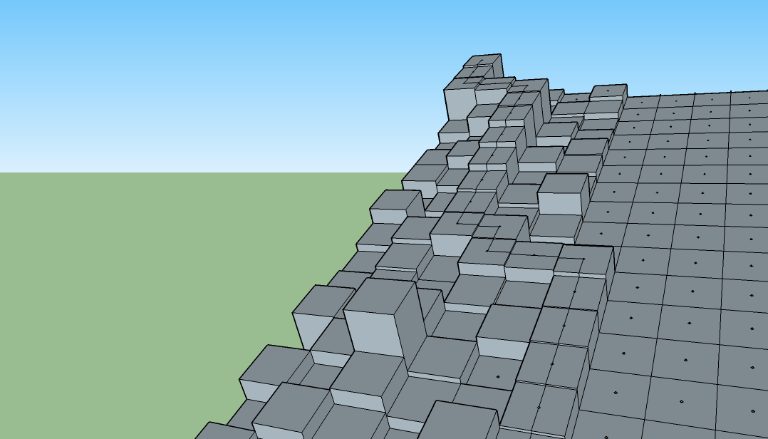
In this report, the field data comes from natural conditions in Japan; the experimental data is obtained from University of Tsukuba Large Rainfall-Simulation Facility. The field is divided into a 24*49 grid. The following section will present the input settings under different conditions. The result will be presented in Chapter 3. All figures and graphs are captured at the scale of 1:43,627,178. Table 1 shows the input settings are modified in this report. In ‘input.dat’ file, the running method of MAHLERAN can be changed by overwriting the symbolic number.
Table 1. Options of input settings.
MAHLERAN also allows users to choose the required output files in ‘output.dat’. This report will focus on three output files, which are the end topography, the discharge of different slope gradient, and hydrographs.
Without Updating the Topography
When topography is not updated while running MAHLERAN, the Scoging method should be adopted. Therefore, the number of iterations between topography updates will not influence the result. Under this condition, two different combinations are run for a further discussion.
Combination 1
Combination 1 is run to provide a primary comparing scheme for other combinations with topography updating and different flow-routing solution method.
Table 2. Combination 1 input settings.
Combination 2
Combination 2 is run to compare with combination 1 to check the difference of outputs between flow-routing solutions.
Table 3. Combination 2 input settings.
Updating the Topography
When topography is updated while running MAHLERAN, the Crank-Nicolson method should be adopted. Therefore, the number of iterations between topography updates will influence the result (Turnbull, Wainwright, & Braizer 2010).
Combination 3
The aim of combination 3 is to provide a primary comparing data for combinations that are run with updating and compare with combination 1 when topography is not updated.
Table 4. Combination 3 Input settings.
Combination 4
Combination 4 is run to compare other combinations with topography updates aimed at finding the best time steps.
Table 5. Combination 4 input settings.
Combination 5
Combination 5 is run to compare other combinations with topography updates aimed at finding the best time steps.
Table 6. Combination 5 input settings.
Combination 6
Combination 6 is run to compare other combinations with topography updates aimed at finding the best time steps.
Table 7. Combination 6 input settings.
Combination 7
Combination 7 is run to compare other combinations with topography updates aimed at finding the best time steps.
Table 8. Combination 7 input settings.
Combination 8
Combination 8 is run to compare other combinations with topography updates aimed at finding the best time steps.
Table 9. Combination 8 input settings.
Combination 9
Combination 9 is run to compare other combinations with topography updates aimed at finding the best time steps.
Table 10. Combination 9 input settings.
Combination 10
Combination 10 is run to compare other combinations with topography updates aimed at finding the best time steps.
Table 11. Combination 11 input settings.
Combination 11
Combination 11 is run to compare other combinations with topography updates aimed at finding the best time steps.
Table 12. Combination 11 input settings.