Introduction
This paper requires the use of statistical analysis to determine relationships among variables. The primary purpose of such analysis is to obtain answers to the organizational questions that Sun Coast asks in order to improve the company’s operational performance. Specifically, this work involves three types of inferential tests supported by descriptive statistics, namely correlation analysis, regression analysis, and multiple regression analysis. Because the results have critical potential for the company and can be used to improve the organizational agenda significantly, their significance must be supported by statistical evidence (Tenny & Abdelgawad, 2021).
To determine the significance of the constructed models and results, a p-value parameter is used at a significance level of.05. It follows that when the calculated p-value is more significant than.05, the null hypothesis cannot be rejected; the reverse is also true. Choosing a significance level of.05 corresponds to a 5% probability of making an error in detecting significant differences when in fact, there are none: in other words, there is always a probability of making an error of the first kind. For this reason, the results of statistical analyses need to be read carefully and interpreted carefully, as they are expected to be embodied in a company’s realistic environment.
Correlation: Hypothesis Testing
The first part of the general statistical analysis requires a Pearson correlation test to determine the strength and direction of the relationship between two continuous variables. The end result, the correlation coefficient, will show how strongly the two variables are related and the direction of the relationship between them and will demonstrate whether or not the result is significant. Below are the formulations of the two statistical hypotheses that are evaluated in this section on how to perform a correlation analysis.
- Ho1: There is no statistically significant relationship between particulate matter size and employee sick days.
- Ha1: There is a statistically significant relationship between particulate matter size and employee sick days.

As shown in Figure 1, the Pearson correlation coefficient between particle size, in microns, and the average number of sick days for an employee is -.716. A negative value of this coefficient indicates a negative direction of the relationship between the two. In other words, the calculation indicates that an increase in particle size leads to a decrease in the average number of absent days for workers, that is, tiny particles are a predictor of an increase in the number of sick days. The absolute value of the Pearson coefficient is.716, indicating a moderately high value for this relationship. To summarize, Figure 1 corresponds to a moderately high negative correlation between the variables. The coefficient of determination R2, which, according to the results of the calculations, was 0.513, is also subject to discussion. This implies that this model explains up to 51.3% of the variance between the variables, indicating moderate reliability of the model.
Of great importance for the correlation analysis is the coefficient of significance, that is, the p-value. The calculated p-value coefficient is.0000, which corresponds to the critically low value of this parameter. Calculating a specific p-value makes no sense, as it is only necessary to compare this value to a significance level of.05. It is clear that the p-value is significantly less than the critical level of significance (p <.05), from which it follows that there is sufficient evidence to reject the null hypothesis and thus accept the null hypothesis. To summarize this section, it follows from the results that increasing the size of the solids leads to a statistically significant reduction in the number of days an employee misses due to illness.
Simple Regression: Hypothesis Testing
The second part of this paper requires a simple linear regression test to determine if one variable can influence another variable. In fact, the regression test is similar to the correlation test performed because both tests allow testing for a reciprocal relationship between continuous variables. However, unlike Pearson correlation, regression analysis also allows for the construction of a regression equation between the variables, which is used to analyze this relationship in more detail and to predict the values of the factors used. To perform the regression analysis, the following hypotheses were used:
- Ho2: There is no statistically significant relationship between safety training expenditure and lost-time hours.
- Ha2: There is a statistically significant relationship between safety training expenditure and lost-time hours.

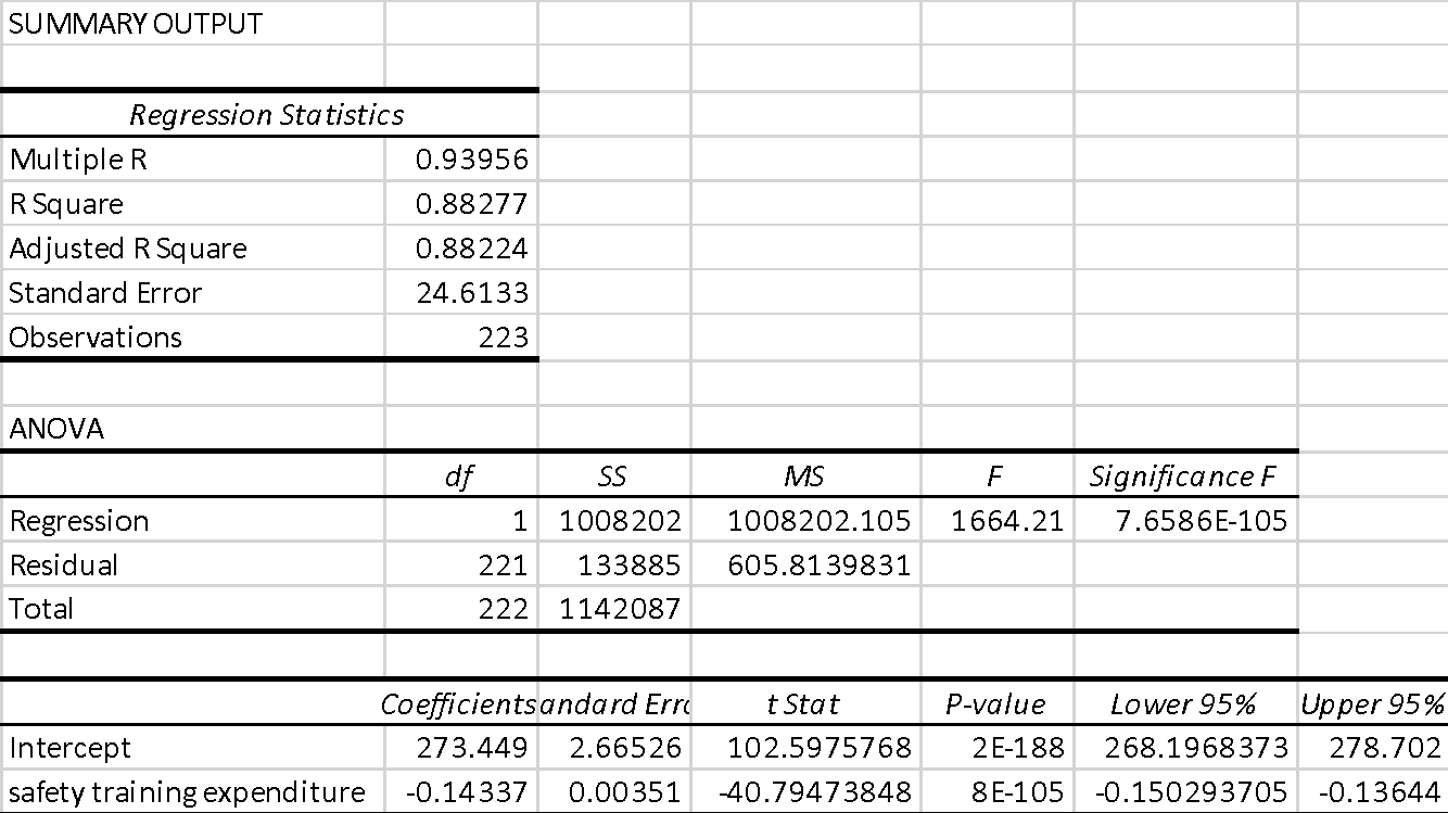
The analysis was performed in MS Excel for the relevant data, and Figure 2 shows the results of these calculations. To check the overall significance of the constructed model, the second table of Fig. 2 is used, namely the results of the ANOVA test. Thus, the overall significance level of the regression model constructed should have been estimated: F(221) = 1664.21, p <.05. This ANOVA data indicates that the model is significant, that is, there is a statistically significant relationship between the tuition expense variables and total hours missed. In other words, the p-value shows that there is sufficient evidence to reject the null hypothesis and accept the alternative hypothesis.
Turning to the third table in Figure 2 provides several conclusions about aspects of this model. In particular, both coefficients — slope and y-intercept — are significant because their respective p-values are well below the critical significance level of.05. This indicates that the regression coefficients are significant, and thus they are reliable parameters for assessing the relationship between variables. In addition, the same table shows that the value of the slope coefficient is -0.143, meaning that there is an inverse relationship between the variables. Increasing the number of training expenditures, it follows, reduces the number of hours workers miss. A regression equation can then be constructed for the data in terms of the variables used, viz:
Lost Time Hours = -0.143*[Safety Training Expenditure] + 273.449
From this equation, in particular, it can be seen that an increase in safety training expenditure for each unit results in a drop of 0.143 hours of lost time. The y-intercept of this equation, that is, the value of the number of hours lost when there is zero investment in training, is also noteworthy. When spending is zero, the number of hours wasted is maximum and is 273.449. When spending increases, there is a downward trend, that is, Sun Coast should be interested in maximizing the amount of reasonable spending to minimize inefficient hours. This equation, among others, is interesting to solve to find the x-intercept.
([Lost Time Hours] – 273.449)/ (-0.143) = [Safety Training Expenditure]
(0 – 273.449)/ (-0.143) = [Safety Training Expenditure]
[Safety Training Expenditure] = 1912.24
This answer shows that with a $1912.24 (in units) investment in safety training, there are zero lost hours for the company, which may be the ultimate goal for organizational reforms at Sun Coast. The coefficient of determination for this regression model and the multiple R are also up for discussion. The coefficient of determination, R2, for this pair of variables is 0.883, indicating that the model covers up to 88.3 percent of the variance between data. This is a high figure, which is consistent with the reliability of the constructed model. The multiple correlation coefficient for these variables was 0.940, which also indicates a strong positive relationship between training costs and hours lost.
Multiple Regression: Hypothesis Testing
In the third part of our work, it was interesting to analyze the effect of different components on the overall perceived noise level. It is known that excessive noise exposure can lead to hearing loss, headaches, and decreased employee productivity (Meersens, 2021). As a consequence, Sun Coast is interested in maintaining acceptable levels of noise exposure to employees and maintaining their operational efficiency. To perform this analysis, several components were used as independent factors, namely frequency, angle in degrees, chord length, velocity, and displacement. Total noise level, measured in decibels, was used as a dependent factor. Since the number of independent factors has been increased, the usual linear regression is no longer applicable to the analysis; instead, multiple regression should be used in MS Excel. Although the steps performed are virtually the same, the results of this analysis will be extended. The following hypotheses are used to run the regression:
- Ho3: There is no statistically significant relationship between frequency, angle in degrees, chord length, velocity, displacement, and decibel level.
- Ha3: There is a statistically significant relationship between frequency, angle in degrees, chord length, velocity, displacement, and decibel level.

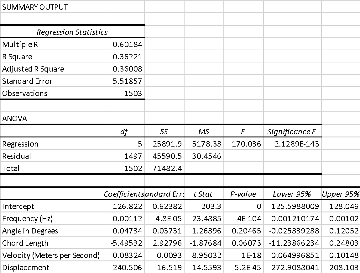
First, it is worth noting that the constructed regression model is statistically significant because the calculated p-value appears to be less than the critical level, F(1497) = 170.036, p <.001. This means that there is sufficient evidence to reject the null hypothesis, which means that the set of independent variables significantly affects the perceived noise level. For the model constructed, the coefficient of determination was 0.362, which implies that about 36.2 percent of the variance between the variables could be explained by the multiple regression model. The correlation coefficient was 0.602, indicating a moderate positive relationship between the two.
Particular attention should be paid to the significance of specific coefficients in the constructed multiple regression model. To be more precise, to evaluate their significance, the null hypothesis is used, that is, the coefficient is equal to zero, that is, it has no influence on the dependent factor. As shown in Table 3 of Figure 3, the p-values were above the.05 significance level only for the Angle and Chord Length variables, which means that these factors had no significant effect on the perceived noise level. In other words, these variables can be omitted in the overall regression equation because they have no significant effect on the noise level. The Frequency, Velocity, and Offset variables were statistically significant because their p-values were below the critical value, so the null hypotheses of no effect were rejected. Thus, the final regression equation in terms of the variables was as follows:
[Decibel] = 126.822 – 0.001*[Frequency] + 0.083*[Velocity] – 240.506*[Displacement]
It follows from the equation that Frequency and Displacement have a negative effect on noise level, that is, their increase led to a decrease in noise level. On the contrary, increasing Velocity increased the perceived noise level. It follows from the results that in order to reduce the overall noise levels perceived by Sun Coast workers, management should increase Frequency and Displacement and decrease Velocity.
Conclusion
In conclusion, this paper conducted statistical analyses — including Pearson correlation, linear regression, and multiple regression — to find answers to Sun Coast’s organizational questions. Particular attention was given to refining statistical significance in the analyses to make sure that the findings actually made sense for further practical implementation. It was found that the smallest particle size was positively correlated with the most extensive employee absences due to illness. This means that company management should keep a close eye on polluting particulate size in an effort to reduce the number of sick leave absences. In addition, increased spending on safety training for employees reduced the number of missed hours. It follows that Sun Coast management should invest more finances in order to increase employee productivity.
Finally, Frequency, Velocity, and Displacement were shown to have differential effects on overall noise levels. Increasing Frequency and Displacement led to a decrease in this parameter, while increasing Velocity led to an increase in noise. Therefore, management should strive to increase Frequency and Displacement and decrease Velocity in order to ensure that the noise level in the company is normal and not destructive to the employees.
References
Meersens. (2021). Noise at work, what impact on the health of employees? Meersens. Web.
Tenny, S., & Abdelgawad, I. (2021). Statistical significance. NIH. Web.