Introduction
Gabriel Cramer (1704-1752) is a familiar name among mathematicians. Cramer was well known for his passion for mathematics such that at his tender age when he was 18 years “he shared a position with Calandrini as the chair in the mathematics department” (Robertson 3). At this stage, Cramer took advantage of his position to travel the world, visiting great mathematicians including Euler, Johann, and Daniel Bernoulli among others. Apart from his academic prowess, he excelled as an editor. One of his popular publications was the “Introduction à l’analyse des lignes courbes algébraique” (Robertson 4). The contents of this book are founded on Newton’s works concerning cubic curves. As such, after introducing Newton’s works, he proceeds to simplify the understanding of these curves in the subsequent chapter. In chapter three, Cramer classifies curves concerning shapes, and it is here that he introduces his famous ‘Cramer’s Rule.’ Here, Cramer applies several arbitrary factors in an equation of the order n, to test his theory. To this end, Cramer “deduces that an equation of degree n can be made to pass through n points” (Robertson 5). To assert his point, Cramer assumes a figure, 5, for n and demonstrates how the equation can be made to cross 5 points. In his solution, Cramer formulates five linear equations and finds a solution using his theory. In this paper, the primary objective is to demonstrate Cramer’s Rule in finding solutions to the two systems given below:
System 1
System 2
Method
According to Cramer, the first step is to transform the linear equations into matrix form.
For system 1, the linear equations take the matrix,

As such, the values for a, b, c and d can be obtained using Cramer’s Rule as per the equations below where the determinant is denoted by the letter D.
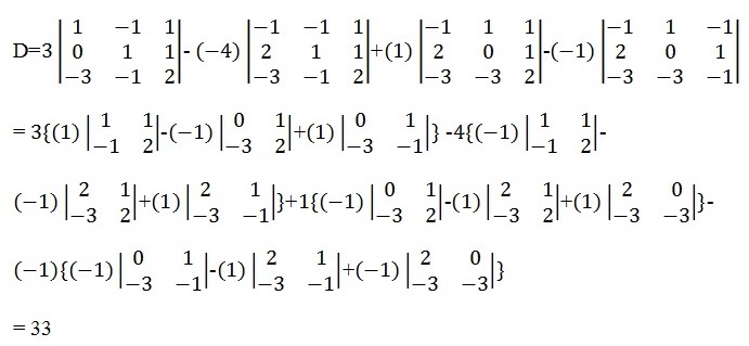
But, D for this matrix is obtained by reducing it from a 4-by-4 to a 2-by-2 matrix as shown below.

Similarly, the value for Da is obtained from the matrix,

Where the first column is replaced by the answer matrix, ![]() , in equation (1) above.
, in equation (1) above.
Therefore,
Da= 33
Thus, a = 1
To obtain Db, the second column is replaced by ![]() This gives;
This gives;

Therefore,
Db= 33
Thus, b= 1
To obtain Db, the third column is replaced by ![]() . This gives;
. This gives;

Therefore,
Dc= 33
Thus, c = 1
To obtain Db, the fourth column is replaced by ![]() . This gives;
. This gives;

Therefore,
Dd= -33
Thus, d = -1
System 2 follows a similar trend. The matrix formation of the linear equations is represented as:

Similarly, the values of p, q, r, and s are obtained using equations 2 above.
Therefore, D = 83
On the other hand, to obtain Dp column 1 is replaced with a matrix ![]() to obtain a matrix,
to obtain a matrix,

Thus, Dp= 166 and,
And, p = 166/83 = 2
To obtain Dq, column 2 is replaced with matrix ![]() to obtain a matrix,
to obtain a matrix,

Thus, Dq= -166 and,
And, q = -166/83 = -2
To obtain Dr, column 3 is replaced with matrix ![]() to obtain a matrix,
to obtain a matrix,

Thus, Dr= 83
And, r = 83/83 =1
To obtain Ds, column 4 is replaced with matrix ![]() to obtain a matrix,
to obtain a matrix,

Thus, Ds=-83
And, s= -83/83 = -1
Conclusion
For system 1, the values for a, b, c, and d are 1, 1, 1, and -1 respectively. On the other hand, for system 2, the values for p, q, r, and s are 2, -2, 1, and -1 respectively. When these values are replaced in the original equations, they confirm Cramer’s Rule as authentic.
Works Cited
Robertson, Fredrick. Mathematicians born in the same country. Logan: Utah State UP, 2015. Print.