Humans make different decisions with regard to the leisure and working time. Indifference curves are commonly used in work-leisure decisions to illustrate the different permutations of income and leisure time that will produce a given level of satisfaction.
This is shown by curve I1 (see figure 1) where the vertical axis measures income level the horizontal axis measures nonmarket activities (leisure). It is worth mentioning that each point on the indifference curve (IC) produces the same level of satisfaction (utility).
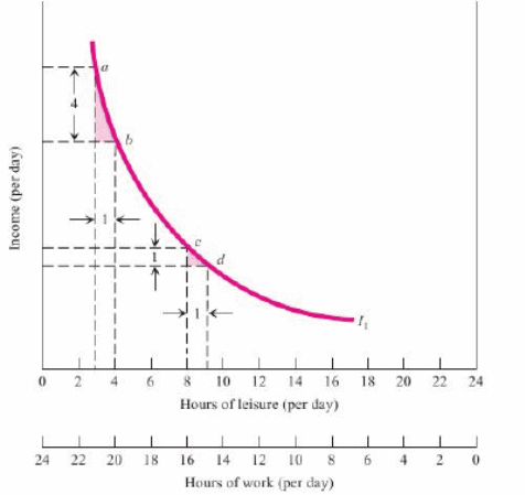
The ICs are convex to the origin because the individual is more unwilling to relinquish their income as it gets scarcer.
Take for example the a-b range of the IC curve (see figure 1), where the person enjoys a moderately large amount of income and very limited leisure time. At this point, the person is ready to substitute 4 units of his/her income for an extra hour of leisure.
The additional satisfaction derived from the extra hour of non-market activity will compensate the satisfaction lost from possessing fewer units (4units) of income. However, if we move to the c-d range (down the IC curve), the income reduces gradually while leisure increases. At this point, the person is ready to substitute one unit of his/her income for an additional hour of leisure.
As the person gains more leisure, the level of income he/she is ready to surrender (to acquire more units of leisure) decreases gradually. In essence, the marginal rate of substitution of leisure for income (MRS L, Y) measures the gradient of the IC.
In other words, the marginal rate of substitution of leisure for income refers to the level of income an individual is willing to surrender to acquire an extra unit of leisure time.
Although an individual aims to maximize his/her satisfaction by shifting to the highest attainable IC, his/her choices are constrained by the amount of disposable income. Let’s assume that work is the only source of income for the individual.
The wage (budget) constraint line (fig. 2) illustrates various income-leisure combinations that an individual can acquire at the stated wage rate. Since the current wage rate is $1, there are two possible combinations for the individual: (1) $24 of income with no leisure; and (2) 24 hours of leisure with no work.
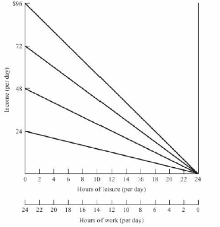
All other feasible options are shown by the line linking these two points (see fig. 2). Since the wage rate is $1, the gradient of the budget line is 1 (see fig. 2).
The individual can obtain maximum satisfaction by combining the objective market data enclosed in each budget line and the personal preferences represented in the ICs (see fig. 3). If the wage rate is $2, the individual cannot attain any leisure-income combination (to the northeast of the resultant HW budget constraint).
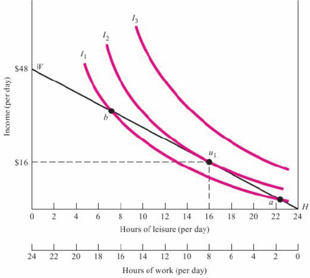
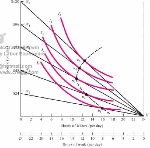
However, the budget constraint permits the individual to obtain maximum level of satisfaction at u1 (where the budget line is tangent to IC I2).
It is obvious that u1produces the maximum attainable level of satisfaction since it lies on the IC (which is furthermost from the origin). Thus, the individual will opt to work for 8 hours (earning $16) and spend 16 hours on leisure.
There are various options an individual might take when the wage rate change. Figure 2 shows that when the wage rates are higher, budget lines become steeper and their contact points with ICs establish various utility-maximizing points.
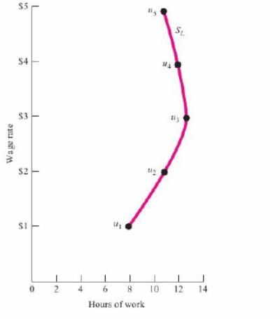
When an individual opts to move from u1to u3 (fig. 4a), it implies that he/she is willing to work for longer hours because the wage rate is higher. Conversely, when he/she shifts from u3 to u5, it means that the individual is willing to work for fewer hours although the wage rate is higher.
Consequently, a backward-bending supply curve emerges (see fig. 4b). Therefore, the supply curve emerges when the individual’s optimal position changes as a result of fluctuations in the wage rates. A backward-bending supply curve results from the income and substitution effects. When the wage rate fluctuates, these two effects can change the utility-maximizing position of an individual.
The income effect indicates a change in the preferred working hours when the income level changes (keeping wage rate constant). Conversely, the substitution effect refers to the adjustment in the preferred working hours when the wage rate changes (holding income constant).
Empirical data suggests that the supply curve for male workers is relatively nonresponsive to alterations in wage rates. Conversely, the labor supply curve for female workers is fairly sensitive to alterations in wage rates. Blundell and McCurdy evaluated 20 studies and reported that when the male wage rates rose by 10%, the quantity of male labor supplied rose by 1%.
Nonetheless, the equivalent figure for female laborers was 8%. It appears that the income effect was higher than the substitution effect for (the male cohort) when the wage rate rose.
On the other hand, the income effect (for the female cohort) was inferior to the substitution effect. The elasticity of labor supply (Es) measures the sensitivity of the level of labor supplied subject to a particular wage rate.
In other words, Es refers to the proportional change in the level of labor supplied divided by the proportional change in the wage rate. Additionally, elasticity is determined by the relative powers of income and substitution effects produced by a change in the wage rate.
Nonparticipants are those people who opt out of the labor force. Figure 5 depicts the characteristics of such individuals. For example, the ICs of nonparticipants are extremely steep. This means that they value leisure more than income. In addition, the MRS L, Y for such individuals is high.
This implies that such people are willing to surrender their income for leisure. Finally, nonparticipant’s NW budget line is relatively even since their wage rates are lower. Figure 5 lends credence to the concept of reservation wage which explains why some people are active in the labor market while others are not.
Therefore, reservation wage refers to the lowest wage rate at which an individual is willing to work. When HN denotes nonparticipant income (see fig. 5), the reservation wage becomes equivalent to the existing market rate (inherent in the broken budget line that is equivalent to the gradient of IC I3).
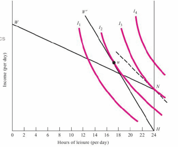
Thus, the value of leisure and the value of work (at the current wage rate) become alike. Consequently, an individual will opt out of the labor force if the reservation wage is above the market wage rate (NW).
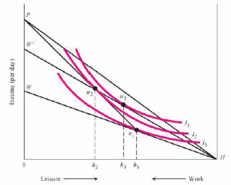
When an employee is compelled to adhere to a standard workday, he/she may be over-employed or underemployed. An employee is deemed over-employed when his/her marginal rate of substitution of leisure for income (for the normal workday) is greater than the wage rate.
On the other hand, an employee is considered underemployed if his/her marginal rate for substitution of leisure for income is less than the wage rate. It is important to mention that the Fair Labor Standards Act [1938] stipulates that a premium wage (particularly time and a half) ought to be paid for the extra labor hours above the 40 hours per week.
As Figure 6 shows, premium wage rate is more conducive for overtime work (Hh2) compared to straight-time wage rate since the latter produces an equal daily income.
There are various income maintenance programs in the United States. Examples of these welfare programs include Medicaid, food stamps, and Supplemental Security Income. These programs have three elementary attributes. These are: (1) The break-even level of income; (2) The benefit reduction rate; and (3) The income basic benefit.
Although these welfare programs have been subjected to criticisms from different quarters, their main goals are to preserve incentives to work, eradicate poverty among poor households, and accomplish the two goals stated above at a sensible cost.
However, the enactment of The Personal Responsibility and Work Opportunity Reconciliation Act (PRWORA) in August 1996 changed the country’s welfare system. Nowadays, the law promotes responsibility with regard to parenthood and encompasses some provisions that reinforce the collection of remittances for child support.
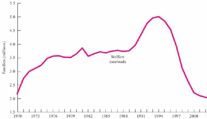
PRWORA has been successful since President Clinton signed it into law. As Figure 7 illustrates, the number of households receiving welfare assistance reduced remarkably from 4.6 million families (in 1996) to approximately 2.1 million families by 2008.
