Introduction
Mathematical modeling of physical processes allows the creation of simulations and prediction of the values of the variables sought, which proves to be particularly useful in the context of engineering tests. One use of simulation is in towing ships, which requires particular sensitivity and reliability (Niklas and Pruszko, 2019). During such a process, the ship is driven by another vessel, which sort of pulls the object along the surface of the water. Obviously, characteristics such as velocity and drag are particularly important since the quality and efficiency of towing is determined by them. The present work does not use a real ship being towed, but instead proposes to perform a simulation on a pool filled with water. Along the long axis of such a pool, the Short and Fat ship model is pulled forward, resulting in a change in velocity over time. It is proposed to study this process mathematically in order to describe any changes that occur to the model. In doing so, it is of great interest to determine the relationship between velocity and time, and to determine the correlation effect between velocity and the R/V variable. This report details the mathematical analysis applied to the data collected and discusses any error limitations.
Experimental Procedure
In a physical test on a pool filled with water, the forced motion of a Short and Fat ship model was observed. During this motion, the velocity of the towed ship was recorded by computer and recorded in data tables. A total of five retests were conducted to minimize errors (Matheson, 2019). A second set was chosen as the optimal set for the present mathematical analysis, which included 571 data points after cutting off unnecessary ends. The values were transferred to an Excel spreadsheet and then statistical analysis was performed, which included creating graphs, calculating the mean and standard deviation, as well as regression analysis. The following sections of this report detail the mathematical procedures that were performed for the data set.
Results and Discussion
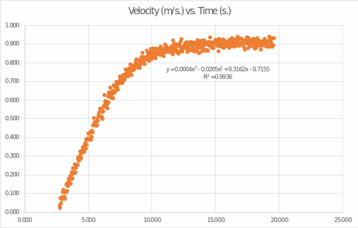
The data used for the mathematical analysis on the second trial, after cutting off the unnecessary ends. These values were used initially to construct a visualization, that is, a scatter plot, in which velocity was plotted on the vertical axis and time on the horizontal axis. This graph is shown in the figure below:

One of the first conclusions that can be drawn from this graph is the nature of the relationship between the two variables. It can be seen that although the velocity increases over time, starting at about the tenth second, its values cease to change significantly. Thus, there is not a linear relationship between the two variables, but rather a polynomial relationship. The regression curve equation shown in this figure describes a third-degree polynomial function. Accordingly, it can be argued that the velocity changes as a function of time according to some polynomial function of the third order. Moreover, this curve is highly consistent because it can cover 99.36% of the variance in the data set (Bloomenthal, 2021). This function can be differentiated to find an expression for the acceleration:
This becomes possible because, as we know, acceleration determines the change in velocity per unit time. The derivative of the velocity function over time is the same, that is, it actually shows the differential of velocity over time. The expression above reflects the quadratic function that describes the change in acceleration for this ship. Similarly, the original function can be integrated to find an expression for the distance traveled:

It follows that the ship covered a distance of 10.04 meters in 19.594 seconds. The upper bound of the integration determines the maximum value of time that was used for the data. Assuming that the same time was used in all tests, and the same force was applied to the towed ship, it becomes clear that all models traveled the same distance. It is noteworthy that such an integration becomes possible at all, since the derivative of distance, that is, the change in distance per unit time, is defined as velocity. Accordingly, the derivative of velocity is distance. In terms of the mathematical meaning of such an integration, the definite integral of the velocity function is equal to the area of the figure which is bounded by the velocity curve and the horizontal axis.
The second part of this report asked us to perform a manual regression analysis for the data set and then compare the resulting equation with the values calculated using Excel. To do this, for each of the five trials, the values of the maximum velocities attained as well as the values of the resistances exerted by the ship in tow were recorded. These data are shown in the table below:
The summing values with the sign ‘Σ’ were calculated as auxiliary coefficients to calculate the regression parameters. This includes both the calculation of the correlation coefficient and the values of the coefficients in the regression equation. To begin with, it was necessary to calculate the correlation between the two variables:
It follows that there is a positive, strong correlation between the two variables (R/V and V). The coefficient R2, which determines the reliability of the regression model, is as follows:
That is, the regression model, which is built next, covers 85.9% of the variance of the data in the set. Actually, to find the coefficients of the equation we need to solve the following equation:
And choose any of the five points to solve the linear equation. The selected point is (0.760, 0.184):
Then the final regression equation takes the form:
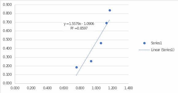
The y-intercept of this function defines a nonzero value of R/V at zero velocity. In fact, this is a semantic error since there is no resistance to towing when there is no motion. The resulting equation can be compared with the automatically calculated one shown in the figure below:

We can see that, in general, the coefficients are close to the automatic calculations. However, due to rounding errors in the calculations shown above, there are errors that result in a slight discrepancy.
In the third part of this report, it was necessary to use the original data, only trimmed so as to leave only 15 values close to the maximum velocity. The following values were used:
Using Excel, the mean value and standard deviation were calculated for fifteen velocity values, which are:
The ratio between them is called SNR and indicates how easy it is to separate the main transmitted signal from the noise. The higher the SNR value, the higher the quality of the signal and the easier it is to use for high-sensitivity data transmission. In this case the SNR equals:
This value defines an excellent SNR level, that is, we can say that this signal is highly sensitive and capable of transmitting information. Therefore, it could be used in telecommunications for the needs of the industry. In terms of mathematical value, this shows that the average value is 50.556 times the standard deviation. That is, the data does not tend to scatter much from the mean, so the signal is excellent.
Finally, in the last part of this report, it was necessary to solve a practical example in which a function for the path is proposed. It is worth saying that all the same concepts and formulas that were used back in Part A are used to solve this scenario. Therefore, this section can be seen as a practice of skills and demonstrations of skills in differentiating and integrating functions. The following function has been proposed as an expression for the distance traveled by the ship:
In the general case, it is again a polynomial function of the third degree, which means that the path as a function of time shows a nonconstant upward trend. From this function, an expression for velocity can be derived by differentiation:
Now the velocity function is already quadratic, which means that the velocity changes according to the parabolic form. In this case, the velocity can increase, fall or be zero, depending on the chosen moment in time. The velocity function can also be used to calculate a particular velocity at a particular point in time:
That is, by the end of the sixth second the ship will have a velocity of 170 m/s. At time t = 1.88 seconds, the velocity is zero:
In fact, the second root of this equation was t = -0.88, but time cannot be negative, so this value was omitted. Similarly, and the velocity function can be differentiated to find an expression for the acceleration:
This is already a linear function, that is, the acceleration for this ship turns out to be constantly increasing. By the end of the fourth second, the acceleration will be:
And at time t = 0.5 seconds, the acceleration was zero:
The path function could also be used to calculate the distance traveled depending on the time value. In particular, by the end of the tenth second, the ship had traveled 1.602 kilometers:
Conclusion
To summarize, this research report investigated the modeling of the Short and Fat ship towing process on a water basin. The data collected were analyzed using integration and differentiation operations as well as through SNR, regression analysis, and graphical representations. The following key findings were made:
- The relationship between velocity and towing time was nonlinear and was determined by the equati

- SNR for velocity values was extremely high and defined a good potential for quality signal transmission.
- There was a strong positive correlation between R/V and V.
- Calculation results did not differ significantly from the Excel output and were due to statistical errors.
Reference List
Bloomenthal, A. (2021) Coefficient of determination. Web.
Matheson, G.J. (2019) ‘We need to talk about reliability: making better use of test-retest studies for study design and interpretation’, PeerJ, 7, pp. 1-10.
Niklas, K. and Pruszko, H. (2019) ‘Full-scale CFD simulations for the determination of ship resistance as a rational, alternative method to towing tank experiments’, Ocean Engineering, 190, pp. 1-8.