Means, Standard Deviations, and Coefficients of Variation
To calculate means and standard deviations, IBM SPSS Statistics can be used. To do so, it is required to select the option to Analyze → Descriptive statistics → Descriptives. In the window that opens, the needed variables should be transferred to the “Variable(s)” box; the button “Options” permits to choose the required statistics (“Mean” and “Std. deviation” should be checked) (George & Mallery, 2016). The syntax is provided in Appendix 1. The results are provided in Table 1 below.
Table 1. Means and standard deviations for the independent variables (exhibitors and sponsors) and the dependent variable (visitors).
Once the means and the standard deviations are known, it is easy to calculate the coefficients of variation by using the following formula (Levine, Stephan, Krehbiel, & Berenson, 2011):
CV = (SD / Mean) × 100%
Therefore,
CV exhibitors = (513.695 / 628.59) × 100% ≈ 81.722%
CV sponsors = (22.466 / 23.29) × 100% ≈ 96.462%
CV visitors = (7254.831 / 7256.41) × 100% ≈ 99.978%
Scatter Plots
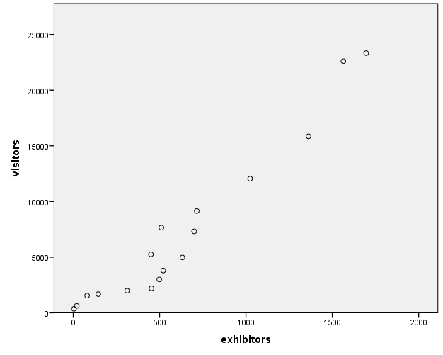
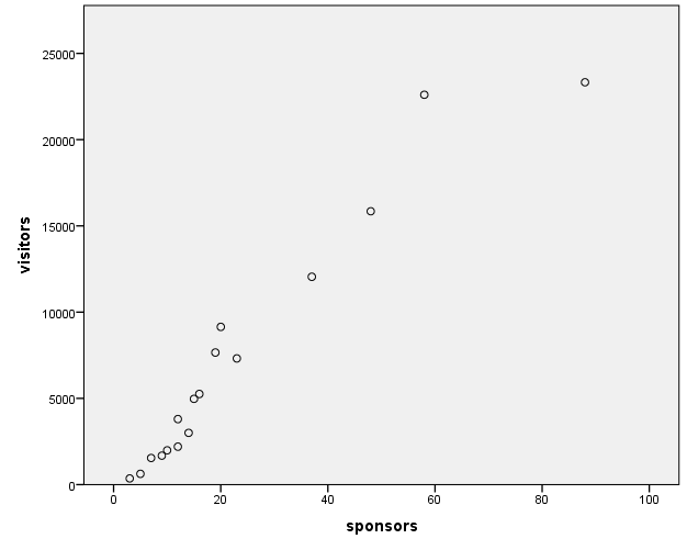
For multiple linear regression, scatter plots are utilized to check the assumption that there is a linear relationship between the dependent and independent variables (Warner, 2013). Therefore, it is needed to create two scatter plots: for exhibitors×visitors and sponsors×visitors.
In SPSS, it is possible to create a scatter plot using the option Graphs → Chart Builder (Field, 2013). In the Chart Builder window, it is required to choose the option “Scatter/Dot” and move the “Simple Scatter” into the preview area. Then, the required variables should be transferred to the respective axes. The SPSS syntax for both scatter plots is supplied in Appendix 2. The results are provided in the figures below.


Correlation Coefficients
In order to obtain Pearson’s correlation coefficients in SPSS, it is required to use the option Analyze → Correlate → Bivariate, and then to transfer all the needed variables into the “Variables” box (George & Mallery, 2016). The SPSS syntax can be found in Appendix 3. The results are shown in Table 2 below.
Table 2. Pearson’s correlation coefficients and their significance.
Linear Regression Equation
To obtain a multiple linear regression equation for the given data, it must first run the numerous linear regression. It can be done using the option to Analyze → Regression → Linear (George & Mallery, 2016). In the Linear Regression window, the variables exhibitors and sponsors should be transferred to the Independent(s) box, whereas the variable visitors should be moved to the Dependent box. It was clicking the Statistics button to choose several options, such as 95% confidence intervals for the regression coefficients. The default method of entering the independent variables into the equation (the process of forced entry) was used.
The syntax for such a regression is given in Appendix 4. The essential output is provided below in Tables 3, 4, and 5.
Table 3. Model summary for the regression.
Table 3 above shows that R2 =.961, which means that the model supposedly explains approximately 96.1% of variance in the data.
Table 4. The ANOVA table for the regression.
Table 4 above shows that the model, on the whole, is statistically significant: F (2) = 174.436, p <.0005. Therefore, it is possible to create a linear regression equation.
Table 5. The regression coefficients output.
As can be seen from Table 5, the Constant coefficient for the overall regression model is not statistically significant: p =.140; therefore, it will not be included into the model. On the other hand, the coefficient b = 7.702 for exhibitors is statistically significant at α =.05: p =.005, so it should be included in the model. Also, the coefficient b = 144.787 for sponsors is statistically significant at α =.05: p =.005, so it should be included in the model as well.
Therefore, the linear regression equation for this model will be as follows:
visitors = (7.702 × exhibitors) + (144.787 × sponsors)
Testing Hypotheses for the Variables
The output for the linear regression, which is provided above in Table 5, permits for testing the null and the alternative hypotheses for the independent variables, exhibitors and sponsors (Dewhurst, 2006).
The null hypothesis for the exhibitors variable can be formulated as follows: “The number of exhibitors at an exhibition cannot be used so as to predict the number of visitors at that exhibition.” The corresponding alternative hypothesis can be formulated as follows: “The number of exhibitors at an exhibition can be used so as to predict the number of visitors at that exhibition.” If α =.05 is set, then the results of the regression permit for rejecting the null hypothesis, and for stating that evidence has been found to support the alternative hypothesis (Render, Stair, Hanna, & Hale, 2015).
The null hypothesis for the sponsors variable can be stated as follows: “The number of sponsors of an exhibition cannot be used in order to predict the number of visitors at that exhibition.” The corresponding alternative hypothesis can be formulated as follows: “The number of sponsors of an exhibition can be used in order to predict the number of visitors at that exhibition.” If the level of alpha is set at α =.05, then the calculations for the regression allow for rejecting the null hypothesis, and for stating that evidence has been found so as to support the alternative hypothesis (Swift & Piff, 2014).
Comments
Variables
The number of exhibitors and the number of sponsors were chosen as independent variables, whereas the number of visitors was selected as dependent variables. This is because it may be assumed that the number of exhibitors (and, therefore, the assortment, for instance) and the number of sponsors (and, therefore, the amount of advertisement, or the overall quality of an exhibition, for example) might have an impact on the number of visitors.
Graphs
The graphs demonstrate that the values of all the considered values, on the whole, grew gradually. However, there were several decreases; for instance, the number of visitors dropped in 2009 (5256 visitors) when compared to 2008 (7316 visitors), but then it started growing again. The number of exhibitors also dropped in 2009 (450 exhibitors) when compared to 2008 (700 exhibitors), but then it also started growing gradually.
Means, Standard Deviations, and Coefficients of Variation
The table shows that SD exhibitors = 513.695, SD sponsors = 22.466, SD visitors = 7254.831. Importantly, such a large difference in variances of exhibitors and sponsors is likely to be troublesome, because it means that the assumption of homogeneity of variances for the regression is probably violated, which might result in inaccurate standard errors and confidence intervals, and biased p-values (Field, 2013).
The coefficients of variation show that, with respect to the mean, the number of exhibitors demonstrates the least variability (CV = 81.72%), whereas the number of sponsors and the number of visitors demonstrate roughly similar variabilities (CV = 96.46% and CV = 99.98%, respectively) which are higher than that of the number of exhibitors (Levine et al., 2011).
Scatter Plots
Both scatter plots apparently show that there are no non-linear relationships between the plotted variables; however, linear relationships are present. This means that the assumption of linear relationships between the dependent variable and each of the independent variables has not been violated (Warner, 2013).
Correlation Coefficients
The correlation coefficients between the variables demonstrate that there exist some serious problems with multicollinearity in the data. It can be seen that Pearson’s r are equal to.947,.970, and, 965 for exhibitors×sponsors, exhibitors×visitors, and visitors×sponsors, respectively, and all of them are significant at α =.01.
According to Field (2013), if the correlation coefficients are higher than.80, then the assumption of non-multicollinearity is violated, which is the case in the analyzed data. It is stated that three main problems might result from this violation: 1) the b coefficients are unreliable and more variable across different samples (which makes the regression equation also untrustworthy); 2) it limits the size of unique variance explained by each of the dependent variables; and 3) it works as a barrier to assessing the individual importance of dependent variables (i.e., if they correlate highly, they may be interchangeable, and it is hard to understand what contribution each one of them does) (Field, 2013).
Linear Regression Equation
Table 5 demonstrates that both independent variables significantly (at α =.05) predicted the dependent variable. This yielded the linear regression equation, which was provided above.
However, it is paramount to stress that there exist a number of concerns that undermine the trustworthiness of this model. It has already been stated that the assumption of homoscedasticity was probably not met and that the assumption of non-multicollinearity was also violated. In addition, the independent variables correlate very highly with the dependent variable, and Table 3 (model summary) shows that the model supposedly explains about 96% of the variance, which may seem suspicious given the nature of the data (because it means that the number of sponsors and the number of exhibitors explain 96% of the variance in the number of the visitors of an exhibition). Also, there might be significant outliers in the data (for instance, sponsors = 88 in 2015 is beyond 2.5 standard deviations from the mean for this variable), and the normality of
References
Dewhurst, F. (2006). Quantitative methods for business and management (2nd ed.). New York, NY: McGraw-Hill.
Field, A. (2013). Discovering statistics using IBM SPSS Statistics (4th ed.). Thousand Oaks, CA: SAGE Publications.
George, D., & Mallery, P. (2016). IBM SPSS Statistics 23 step by step: A simple guide and reference (14th ed.). New York, NY: Routledge.
Government of Dubai. (2017). Wetex 2016 – facts and figures. Web.
Levine, D. M., Stephan, D. F., Krehbiel, T. C., & Berenson, M. L. (2011). Statistics for managers using Microsoft Excel (6th ed.). Upper Saddle River, NJ: Pearson Prentice Hall.
Render, B., Stair, R. M., Hanna, M. E., & Hale, T. S. (2015). Quantitative analysis for management (12th ed.). Harlow, UK: Pearson Prentice Hall.
Swift, L., & Piff, S. (2014). Quantitative methods for business, management & finance (4th ed.). New York, NY: Palgrave Macmillan.
Warner, R. M. (2013). Applied statistics: From bivariate through multivariate techniques (2nd ed.). Thousand Oaks, CA: SAGE Publications.