Algebra: Y-Intercept and X-Intercept Coursework

Intercepts and What it means when a Line Has No Y-Intercept or No X-Intercept

In graphing, we always talk about the x-intercept and the y-intercept. According to Seward (2011), intercepts are special types of solutions to algebraic equations. Intercepts may also be regarded as intersects or locations where the graph crisscrosses the x-axis or y-axis. The x-intercept is where the graph crosses the x-axis while the y-intercept is where the graph crosses the y-axis (Seward, 2011).

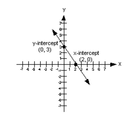
Based on the above descriptions, the value of y will always be 0 regardless of where one is on the x-axis. Similarly, the value of x will always be 0 at any point along the y-axis. The graph in figure 1 below shows the x and y-intercepts.

The x-intercept is the point (2, 0) along the x-axis and the y-intercept is the point (0, 3) along the y-axis. It is important to note that the x and y-intercepts are two separate points on the graph and the only time when both the x and y-intercepts will be the same is at point (0, 0) which is the origin.

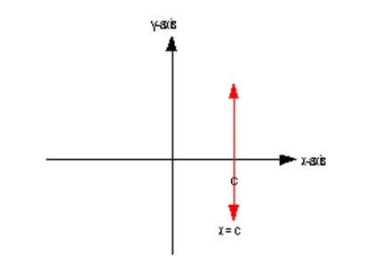
Looking at the graph in figure 1, when a line does not have a y-intercept, it means that is a vertical line parallel to the y-axis. The line only crosses the x-axis and the value of x is a constant. This is illustrated by figure 2.

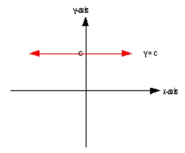
On the other hand, when a line is without an x-axis, then the line is horizontal and parallel to the x-axis. This line only cuts through the y-axis and the value of y is a constant. This is illustrated by figure 3.

Example of a Real-Life Situation Where a Graph Would Have No X- or Y-Intercept

A real-life situation where a graph will have no x or y-intercept is a case that gives a constant solution. A good example is the rate at which a human being’s heartbeats. Usually, the rate of the heartbeat is constant. This may, however, not be the case at all times considering that in some situations the rate at which the heart beats will vary. An example is when the rate of the heartbeat is taken after one has been subjected to vigorous exercise. Heartbeat rates taken at this moment will vary greatly.

Concept of Modeling

Mathematical modeling refers to the use of mathematics to describe real-world situations using mathematical equations. Using models an experimenter can investigate issues about observations and make future predictions concerning a real-world environment. Various concepts may also be tested using mathematical models (DeVries, n.d). An algebraic equation is one of the very useful tools that can be applied in a modeling process.

Describing Known Data Using a Model and Predicting Future Data

In describing known data, a model will make use of algebraic equations. Instead of carrying out experiments in the real world, the use of models allows the experimenter to do experiments based on mathematical representations of the real world rather than facts (DeVries, n.d).

The modeling process has four distinct stages. First, data is collected from the real world. Next, the data is formulated into a model which is then used by the experimenter to do an analysis and produce mathematical conclusions. Finally, the mathematical conclusions are interpreted to predict or explain future behavior (DeVries, n.d).

How do Models Breakdown?

Many experimenters have argued that models will break down when they are used beyond a certain time limit. However, this depends very much on the type of data and subject matter under investigation.

Example of Mathematical Modeling around Us all of the Time

All around us, we are surrounded by numerous examples of mathematical modeling. Suppose that teachers in a high school are not satisfied with their pay and decide to go on strike. We may be interested to determine the effect of such a strike on the overall student performance.

References

DeVries, G. (n.d). What is Mathematical Modeling? Alberta, CA: University of Alberta. Web.

Seward, K. (2011). Intermediate Algebra Tutorial 14: Graphing Linear Equations.Canyon, TX: West Texas A&M University. Web.