Summary
A department dealing with the effects of atmospheric pollutants in the vicinity of an industrial complex has established a data table of measurements of a purity index Y on a scale of 0 (extremely bad ) to 1000 ( absolutely pure) and the dependence of this on component pollutant variables X1, X2, …, X6. The aim of the department is to establish which of the component variables is contributing most to local atmospheric pollution.
This report analyzed and discussed the association of the purity index Y with component pollutant variables and developed a model to forecast the purity index. The analysis suggested that the component pollutant variables X1, X2, X4, X5, and X6 are significantly related to purity index Y (p <.05). However, only two-component pollutant variables X1 and X5 are most likely to contribute significantly to atmospheric pollution (purity index Y). The equation for the best regression (chosen) model was given by Y = 0.185 + 1.111X1 + 7.598X5
Further, for the chosen model, all the underlying assumptions of the regression analysis (multicollinearity, non-normality, nonconstant variance, and autocorrelation) are valid.
Introduction
A department dealing with the effects of atmospheric pollutants in the vicinity of an industrial complex has established a data table of measurements of a purity index Y. The purity index Y is measured on a scale of 0 to 1000, with 0 being extremely bad and 1000 being absolutely pure and the dependence of this on component pollutant variables X1, X2, …, X6. The aim of the department is to establish which of the component variables is contributing most to local atmospheric pollution.
This report will analyze and discuss the association of the purity index Y with component pollutant variables X1, X2, …, X6. Further, this report will develop a model for forecasting the purity index Y based on component pollutant variables X1, X2, …, X6. For this, sample data for a period of 50 days is obtained. The test is a ‘blind’ one in the sense that none of the pollutants has been identified by name, because of its association with the source and the possibility at this stage of unwanted litigation.
Correlation and Scatterplot Analysis
Figure 1 to 6 shows the scatterplots of purity index Y against component pollutant variables X1, X2… X6.
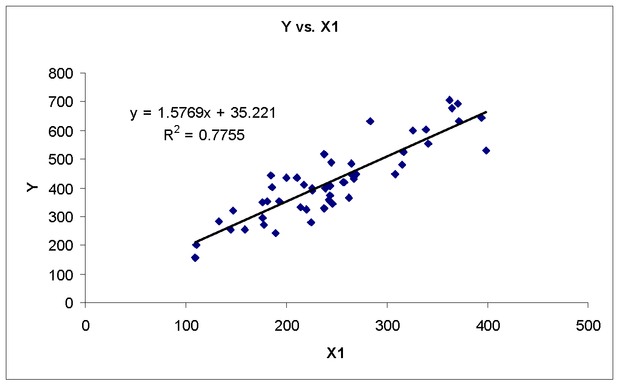
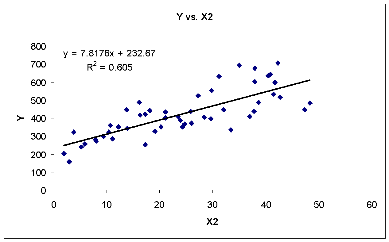
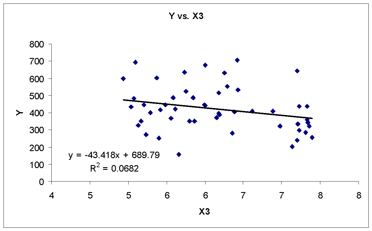
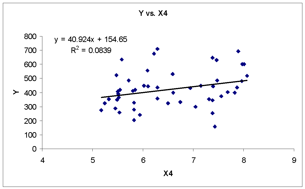
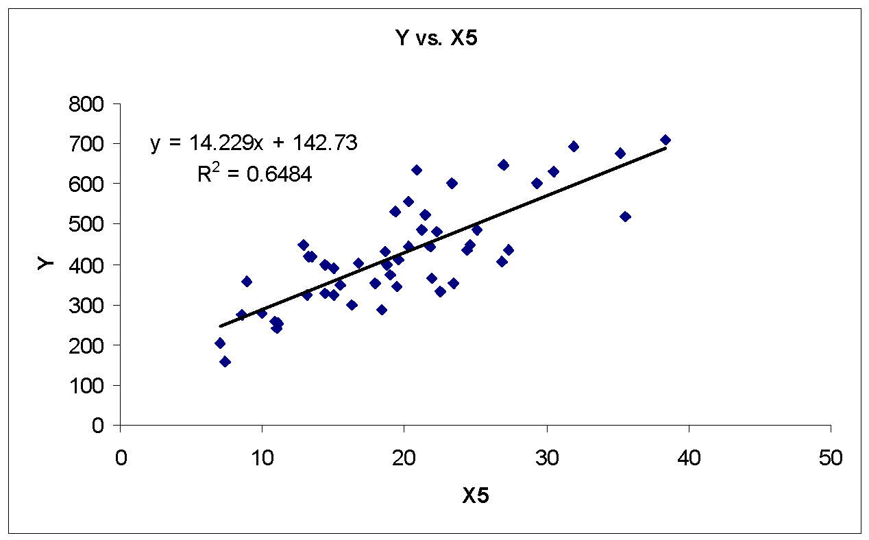
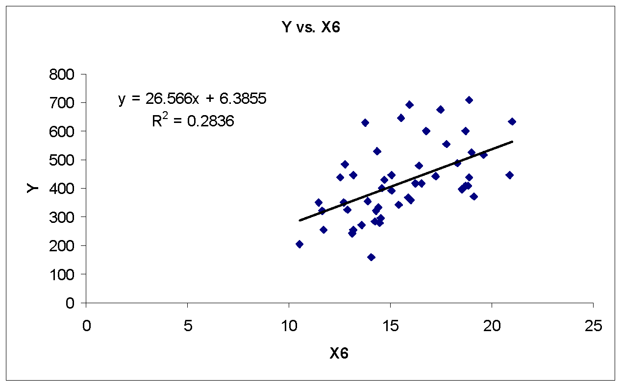
There appears a strong linear relationship between Y and X1, Y and X2, and Y and X5. In addition, there appears a moderately strong linear relationship between Y and X6. Furthermore, there appears weak or no linear relationship between Y and X3 and Y and X4. Table 2 shows the correlation matrix (using MegaStat, an Excel Add-in) for purity index Y and component pollutant variables X1, X2… X6.
Table 1: Correlation Matrix
As shown in table 1, the correlation of Y is significant for X1, X2, X4, X5, and X6. Therefore, excluding component pollutant variable X3 from first multiple regression analysis based on correlation and scatterplot analysis.
Multiple Regression Model
Model with Five Independent Variables (Excluding X3)
Table 2
Table 2 shows the regression model with five component pollutant variables. Although, the regression model is significant (F = 77.64, p <.001), the p-value for coefficient of component pollutant variables X2, X4, and X6 are greater than 0.05. The p-value for coefficient of X6 (0.462) is higher as compared to coefficient of other component pollutant variables X2 (0.188) and X4 (0.3868), thus, excluding component pollutant variable X6 from further multiple regression analysis.
Model with Four Independent Variables (Excluding X3 and X6)
Table 3
Table 3 shows the regression model with four component pollutant variables. Although, the regression model is significant (F = 97.90, p <.001), the p-value for coefficient of component pollutant variables X2 and X4 are greater than 0.05. The p-value for coefficient of X4 (0.443) is higher as compared to coefficient of component pollutant variable X2 (0.265), thus, excluding component pollutant variable X4 from further multiple regression analysis.
Model with Four Independent Variables (Excluding X3, X4 and X6)
Table 4
Table 4 shows the regression model with three component pollutant variables. Although, the regression model is significant (F = 131.35, p <.001), the p-value for coefficient of component pollutant variable X2 (0.287) is greater than 0.05, thus, excluding component pollutant variable X2 from further multiple regression analysis.
Model with Two Independent Variables X1 and X5
Table 5
Table 5 shows the regression model with two component pollutant variables X1 and X5. The regression model is significant (F = 195.77, p <.001). The p-value for coefficient of component variables X1 and X5 is significant that indicates that both component pollutant variables X1 and X5 significantly predicts purity index Y in regression model.
Table 6 shows the stepwise regression (using MegaStat, an Excel Add-in) taking n number of variables (best for n). As shown in table 6, the best multiple regression model is given by component pollutant variables X1 and X5, as p-value for model is highest.
Table 6: Multiple regression model with different number of independent variables
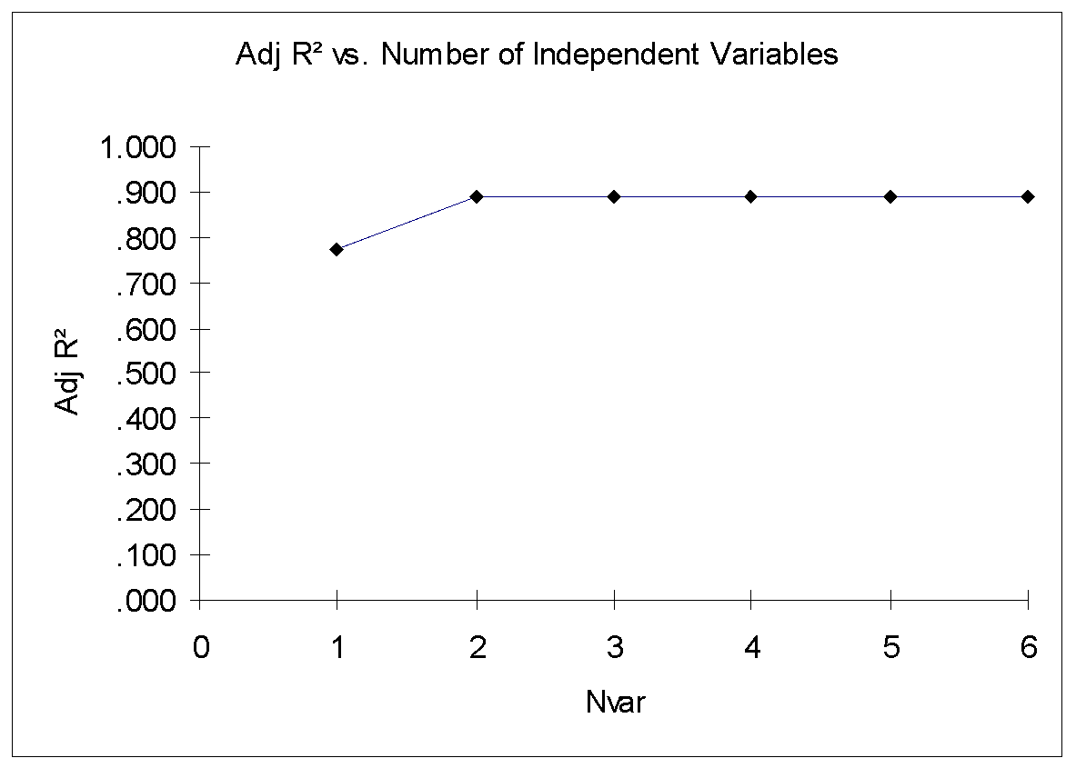
Adjusted R2 is a parameter for deciding number of independent variables in multiple regression model. Figure 7 show the Adjusted R2 versus Number of Independent Variables. As shown in figure 7, there is not much increase in Adjusted R2 after two independent variables X1, and X5. The Adjusted R2 value is approximately same (0.888) for more than 2 independent variables in multiple regression model. Therefore, the best regression model is given by only taking two independent variables X1, and X5.
Chosen Multiple Regression Model
The equation for the best regression (chosen) is given by Y = 0.185 + 1.111X1 + 7.598X5
Regression slope coefficient of 1.111 of X1 indicates that for each point increase in X1, purity index Y increase by about 1.111 on average given fixed component pollutant variable X5.
The regression slope coefficient of 7.598 of X2 indicates that for each point increase in X2, purity index Y increase by about 7.598 on average given fixed component pollutant variable X1.
Component pollutant variables X1 and X5 explain about 89.3% variation in purity index Y. The other 10.7% variation in purity index Y remains unexplained may be due to other factors.
T-tests on Individual Coefficients
The null and alternate hypotheses are:


The selected level of significance is 0.05 and the selected test is t-test for Zero Slope.
The decision rule will reject H0 if p-value ≤ 0.5. Otherwise, do not reject H0.
Component pollutant variable X1 significantly predicts purity index Y, t(47) = 10.35, p <.001.
Component pollutant variable X5 significantly predicts purity index Y, t(47) = 7.17, p <.001.
F – test on All coefficients
The null and alternate hypotheses are:


The selected level of significance is 0.05 and the selected test is F-test.
The decision rule will reject H0 if p-value ≤ 0.5. Otherwise, do not reject H0.
The regression model is significant, R2 =.893, F(2, 47) = 195.77, p <.001.
Assumptions of Regression Model
Multicollinearity
Klein’s Rule suggests that we should worry about the stability of the regression coefficient estimates only when a pairwise predictor correlation exceeds the multiple correlation coefficient R (i.e., the square root of R2). The value of the correlation coefficient between X1 and X5 is 0.605. The value of Multiple R for the final regression model with X1 and X5 is 0.945 and far exceeds 0.605, which suggests that the confidence intervals and t-tests may not be affected.
Another approach for checking multicollinearity is the Variance Inflation Factor (VIF). Figure 2 shows the interpretation of the Variance Inflation Factor (VIF). As a Rule of Thumb, we should not worry about multicollinearity, if VIF for the explanatory variable is less than 10.
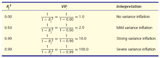
Table 7: Variance Inflation Factor (VIF) using MegaStat
As shown in table 7, the VIF’s for both X1 and X5 is 1.576; thus, there is no need for concern.
Non-Normal Errors
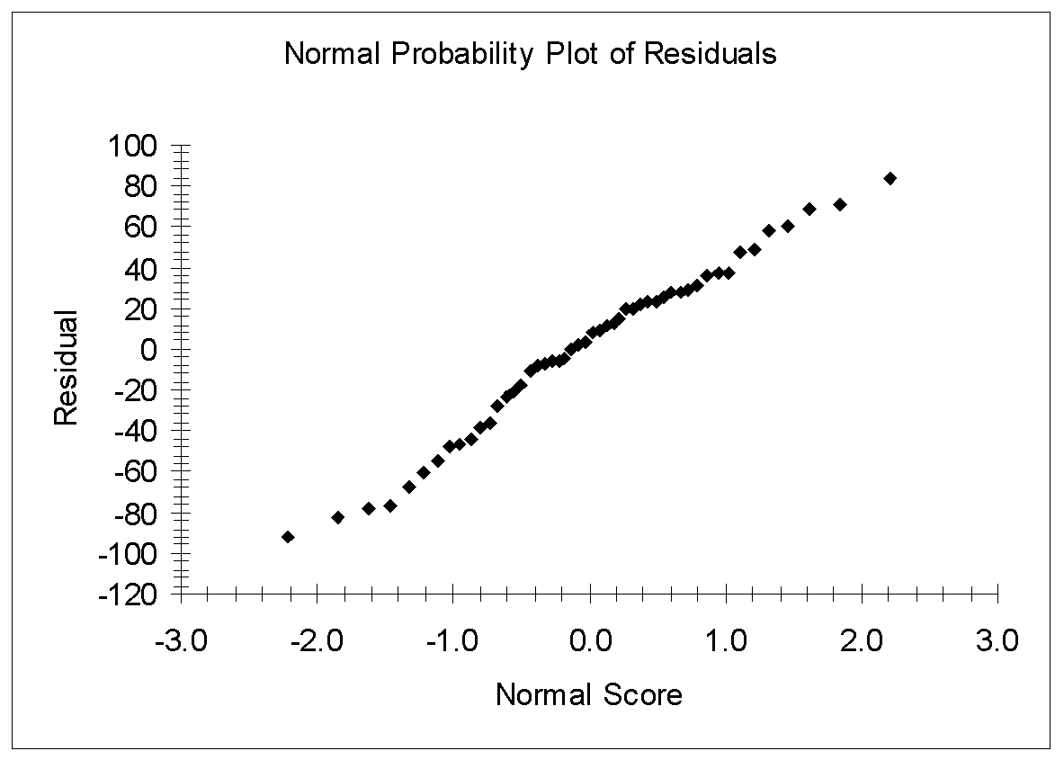
Figure 9 shows the normal probability plot of residuals. As shown in figure 9, the residual plot is approximately linear, thus, the residuals seem to be consistent with the hypothesis of normality.
Nonconstant Variance (Heteroscedasticity)
Figure 10 and 11 show the plots of residuals by X1 and residuals by X5.
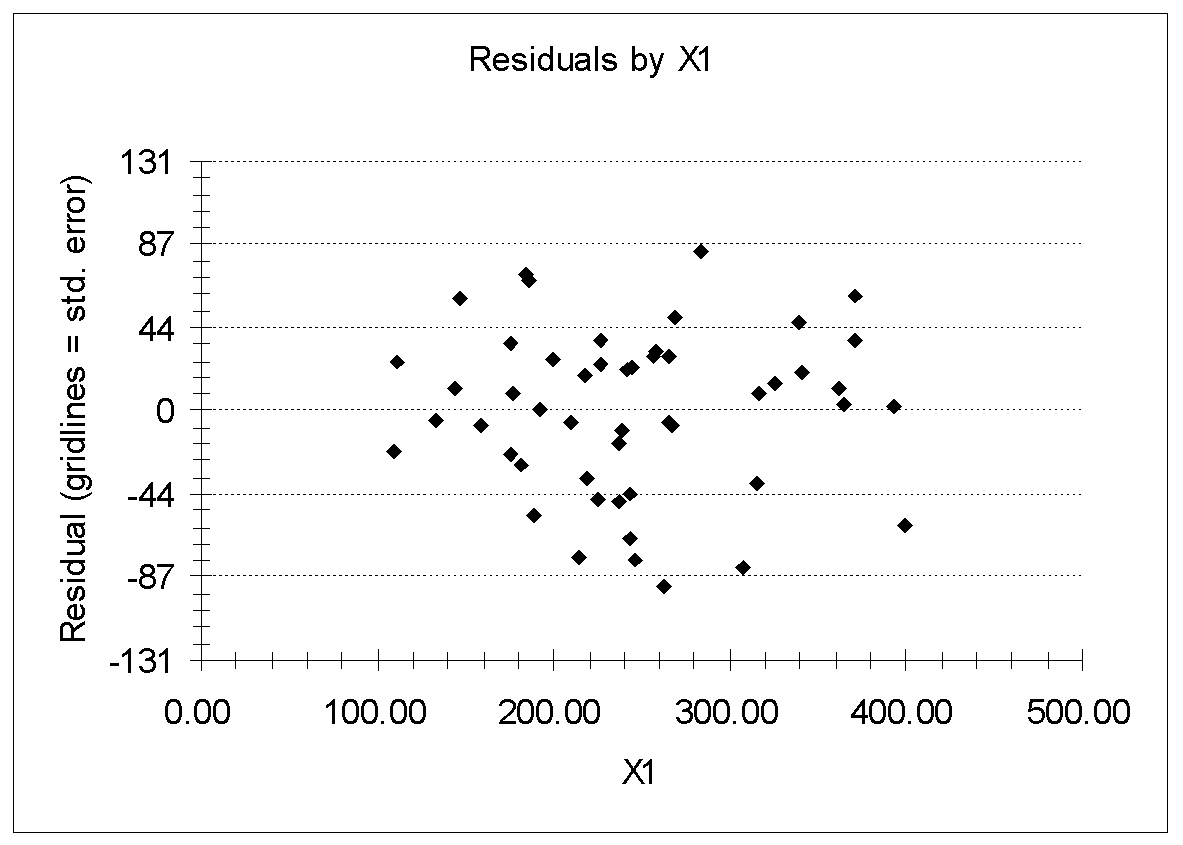
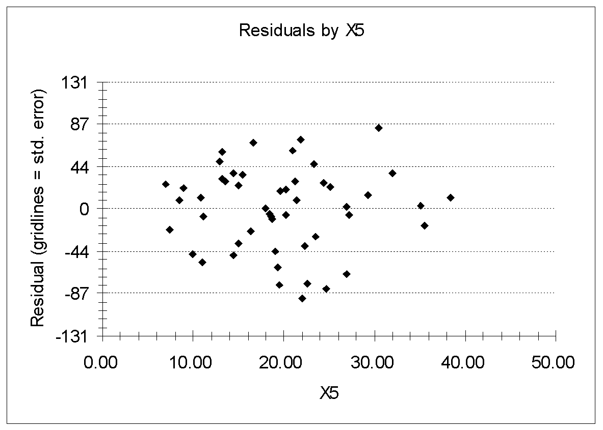
As shown in figure 10 and 11 the data points are scattered, and there is no pattern in the residuals as we move from left to right, thus, the residuals seem to be consistent with the hypothesis of homoscedasticity (constant variance).
Autocorrelation
Autocorrelation exists when the residuals are correlated with each other. With time-series data, one needs to be aware of the possibility of autocorrelation, a pattern of nonindependent errors that violate the regression assumption that each error is independent of its predecessor. The most common test for autocorrelation is the Durbin-Watson test. The DW statistic lies between 0 and 4. For no autocorrelation, the DW statistic will be near 2. In this case, DW = 2.33, which is near 2, thus errors are non-autocorrelated. However, for cross-sectional data, the DW statistic is usually ignored.
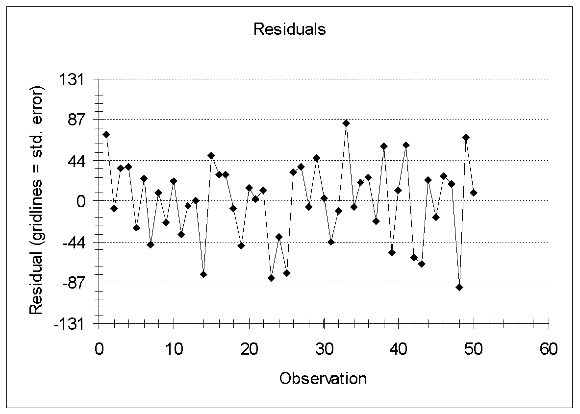
Figure 12 shows the residual by observation number. As shown in figure 12, the sign of a residual cannot be predicted from the sign of the preceding one this means that there is no autocorrelation.
Thus, for the chosen model, all the underlying assumptions of the regression analysis are valid.
Pollutant Variables (X) to Contribute Atmospheric Pollution (Purity Index Y)
As shown in table 1: correlation matrix, the component pollutant variables X1, X2, X4, X5, and X6 are significantly related to purity index Y (p <.05). Thus, they all are individually contributing significantly to atmospheric pollution. However, looking at the multiple regression model analysis, the only two-component pollutant variables X1 and X5 are most likely to contribute significantly to atmospheric pollution (purity index Y).