Building a Cox Proportional Hazards Model Coursework

Exclusively available on Available only on IvyPanda® Written by Human No AI

Identifying the Variables

In the given dataset, the censoring variable will be stroke, because the cases will be censored according to it; the cases will be right-censored if stroke=0, i.e. for those patients who did not have a stroke while having been observed.

The time-to-event variable will be followed; it shows how long the patients had been observed before they suffered from a stroke or withdrew from the study (were censored).

Tied events are events which occurred at the same time (Borucka, 2014). As can be seen from the frequency table for the variable followed in Appendix 1, there were no tied events in the data; all the 31 events where followed=32.02 are censored.

For a research question “Is there an association between hypertension and the time a person was followed before experiencing a stroke?,” hypertension is the independent variable.

#VariableRole in the analysis
1strokeCensoring and outcome (dependent) variable
(event variable)
2followedTime-to-event variable
3hypertensionIndependent (covariate), exposure variable

Testing the Assumption of Proportionality Using Kaplan-Meier Method

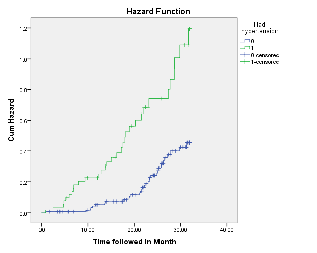
The hazard plot for the given dataset using time=followed, status=stroke, and factor=hypertension, is as follows:
Testing the Assumption of Proportionality Using Kaplan-Meier Method

The plot of hazard functions can be utilized in order to evaluate whether the assumption of proportionality of hazards is violated (Forthofer, Lee, & Hernandez, 2007).

It appears that the baseline hazards (the blue line, the one which depicts hazards for the group with no hypertension) are proportional to the hazards in the tested group (the green line, which represents hazards for the groups with hypertension) at least at some intervals:

  1. At the interval of time from 0 to approximately 10 months, the hazards do not appear proportional, for the baseline hazards remain constant and very close to 0, while the hazards in the tested group increase;
  2. During the interval of time from nearly 10 to roughly 22 months, the hazards are proportional (apparently), for both lines grow constantly, even though the hazards in the tested group grow faster;
  3. During the interval of time from approximately 22 to 32.02 months, the hazards also seem to be proportional, although the proportion appears to differ from that which held in the previous interval, for the hazards in the tested group go up considerably faster.

If the hazards are proportional in both the test/experimental group and the baseline group, it means that the assumption of proportional hazards is satisfied, and the Cox proportional hazards model can be built; there is no need to look for alternative tests or to try to adjust the test (Forthofer et al., 2007).

The Cox Proportional Hazards Test

Reporting and Interpreting the Test

The results of the test (time = followed, status = stroke, covariates = hypertension(Cat)) are as follows:

Categorical Variable Codingsa
Frequency(1)c
Had hypertensionb01251
1550
a. Category variable: Had hypertension (hypertension)
b. Indicator Parameter Coding
c. The (0,1) variable has been recoded, so its coefficients will not be the same as for indicator (0,1) coding.
Omnibus Tests of Model Coefficients
-2 Log Likelihood
609.936
Case Processing Summary
NPercent
Cases available in analysisEventa6536.1%
Censored11563.9%
Total180100.0%
Cases droppedCases with missing values00.0%
Cases with negative time00.0%
Censored cases before the earliest event in a stratum00.0%
Total00.0%
Total180100.0%
a. Dependent Variable: Time followed in Month
Omnibus Tests of Model Coefficientsa
-2 Log LikelihoodOverall (score)Change From Previous StepChange From Previous Block
Chi-squaredfSig.Chi-squaredfSig.Chi-squaredfSig.
592.01220.7261.00017.9241.00017.9241.000
a. Beginning Block Number 1. Method = Enter
Variables in the Equation
BSEWalddfSig.Exp(B)95.0% CI for Exp(B)
LowerUpper
Had hypertension-1.081.24918.8521.000.339.208.553

Therefore, the variable hypertension significantly predicted the difference in survival (that is, in the occurrence of a stroke): B(1)=-1.081, p<.001. Therefore, the hazard ratio based on the variable hypertension was: Exp(B)=.339 (95% confidence interval:.208-.553), which means that for a patient without hypertension, the stroke hazard is approximately.339 times of that of a patient with hypertension.
The Cox Proportional Hazards Test

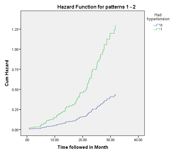
The hazard plot shows the change in cumulative hazard of stroke for groups with and without hypertension with the passage of time. The horizontal axis shows time, whereas the vertical axis shows the cumulative hazard, which equals to the negative log of probability of survival (Forthofer et al., 2007). Clearly, the hazard grows considerably faster in the group with hypertension.

Effects of the Presence of Ties

It is stressed that while calculating the partial likelihood function, the order in which events occur plays an important role, because each time an event takes place, certain expressions describing the states of all the subjects that are at risk at the time of that event are added; therefore, if two events are tied, it is not clear which of the participants should be considered having an event, and which ought to be counted as being at risk (Borucka, 2014, p. 95). This hinders the calculation of the partial likelihood function (Borucka, 2014).

To address the problem of ties, Borucka (2014) offers five different methods, the simplest of which is subtracting a very small random number from the time of tied events (it is stated to be quite effective), two more complicated ones are Efron and Breslow approximations (Efron approximation is claimed to be better), whereas the discrete model and the exact expression are the methods which are argued to result in the best model fit but are cumbersome.

References

Borucka, J. (2014). Methods for handling tied events in the Cox proportional hazard model. Studia Oeconomica Posnaniensia, 2(2), 91-106. Web.

Forthofer, R. N., Lee, E. S., & Hernandez, M. (2007). Biostatistics: A guide to design, analysis, and discovery (2nd ed.). Burlington, MA: Elsevier Academic Press.

Appendix 1

Frequencies table for the variable followed:

Time followed in Month
FrequencyPercentValid PercentCumulative Percent
Valid.821.6.6.6
.901.6.61.1
1.671.6.61.7
2.481.6.62.2
3.431.6.62.8
3.811.6.63.3
3.831.6.63.9
3.851.6.64.4
4.041.6.65.0
4.631.6.65.6
4.781.6.66.1
4.861.6.66.7
5.261.6.67.2
5.511.6.67.8
5.551.6.68.3
5.881.6.68.9
5.991.6.69.4
6.631.6.610.0
6.911.6.610.6
6.931.6.611.1
6.991.6.611.7
8.041.6.612.2
9.361.6.612.8
9.571.6.613.3
9.631.6.613.9
9.821.6.614.4
9.881.6.615.0
10.541.6.615.6
10.641.6.616.1
11.011.6.616.7
11.621.6.617.2
11.711.6.617.8
11.781.6.618.3
12.081.6.618.9
12.141.6.619.4
12.231.6.620.0
12.851.6.620.6
13.671.6.621.1
13.781.6.621.7
13.791.6.622.2
13.801.6.622.8
14.011.6.623.3
14.091.6.623.9
14.151.6.624.4
15.101.6.625.0
15.631.6.625.6
15.911.6.626.1
16.281.6.626.7
16.291.6.627.2
17.171.6.627.8
17.301.6.628.3
17.451.6.628.9
17.521.6.629.4
17.591.6.630.0
17.891.6.630.6
17.951.6.631.1
17.961.6.631.7
18.021.6.632.2
18.311.6.632.8
18.431.6.633.3
18.911.6.633.9
18.931.6.634.4
19.101.6.635.0
19.451.6.635.6
19.581.6.636.1
19.681.6.636.7
20.181.6.637.2
20.271.6.637.8
21.101.6.638.3
21.381.6.638.9
21.561.6.639.4
21.611.6.640.0
21.661.6.640.6
21.661.6.641.1
21.711.6.641.7
21.791.6.642.2
22.071.6.642.8
22.081.6.643.3
22.121.6.643.9
22.211.6.644.4
22.381.6.645.0
22.451.6.645.6
22.581.6.646.1
22.991.6.646.7
23.011.6.647.2
23.171.6.647.8
23.271.6.648.3
23.321.6.648.9
23.401.6.649.4
23.571.6.650.0
24.061.6.650.6
24.201.6.651.1
24.331.6.651.7
24.351.6.652.2
24.421.6.652.8
24.901.6.653.3
25.091.6.653.9
25.161.6.654.4
25.221.6.655.0
25.251.6.655.6
25.331.6.656.1
25.761.6.656.7
25.771.6.657.2
25.841.6.657.8
25.871.6.658.3
25.891.6.658.9
25.931.6.659.4
26.021.6.660.0
26.261.6.660.6
26.291.6.661.1
26.451.6.661.7
26.621.6.662.2
26.811.6.662.8
27.091.6.663.3
27.331.6.663.9
27.371.6.664.4
27.711.6.665.0
27.721.6.665.6
27.731.6.666.1
28.151.6.666.7
28.641.6.667.2
28.671.6.667.8
28.861.6.668.3
29.731.6.668.9
29.811.6.669.4
29.981.6.670.0
30.091.6.670.6
30.341.6.671.1
30.731.6.671.7
30.891.6.672.2
31.011.6.672.8
31.121.6.673.3
31.201.6.673.9
31.271.6.674.4
31.281.6.675.0
31.301.6.675.6
31.331.6.676.1
31.371.6.676.7
31.401.6.677.2
31.471.6.677.8
31.551.6.678.3
31.611.6.678.9
31.631.6.679.4
31.631.6.680.0
31.641.6.680.6
31.721.6.681.1
31.911.6.681.7
31.971.6.682.2
31.981.6.682.8
32.023117.217.2100.0
Total180100.0100.0
More related papers Related Essay Examples
Cite This paper
You're welcome to use this sample in your assignment. Be sure to cite it correctly

Reference

IvyPanda. (2022, September 23). Building a Cox Proportional Hazards Model. https://ivypanda.com/essays/building-a-cox-proportional-hazards-model/

Work Cited

"Building a Cox Proportional Hazards Model." IvyPanda, 23 Sept. 2022, ivypanda.com/essays/building-a-cox-proportional-hazards-model/.

References

IvyPanda. (2022) 'Building a Cox Proportional Hazards Model'. 23 September.

References

IvyPanda. 2022. "Building a Cox Proportional Hazards Model." September 23, 2022. https://ivypanda.com/essays/building-a-cox-proportional-hazards-model/.

1. IvyPanda. "Building a Cox Proportional Hazards Model." September 23, 2022. https://ivypanda.com/essays/building-a-cox-proportional-hazards-model/.


Bibliography


IvyPanda. "Building a Cox Proportional Hazards Model." September 23, 2022. https://ivypanda.com/essays/building-a-cox-proportional-hazards-model/.

If, for any reason, you believe that this content should not be published on our website, please request its removal.
Updated:
This academic paper example has been carefully picked, checked and refined by our editorial team.
No AI was involved: only quilified experts contributed.
You are free to use it for the following purposes:
  • To find inspiration for your paper and overcome writer’s block
  • As a source of information (ensure proper referencing)
  • As a template for you assignment
1 / 1