Cattle products are fascinating and convenient sources of materials and nutrients. Beef and milk are some of the leading products used for food. The skin is mostly used in industries; hence it does not attract a lot of investments. However, people worldwide consume milk and its products and beef daily. Still, there are widespread protein deficiencies in developing countries in which people continue to subsist on starchy diets. Beef and milk are some of the mostly used proteins, which together with other micronutrients such as vitamins and calcium, are critical elements needed by all. Consequently, cattle farming has been one of the main areas of attractive areas in agribusiness, particularly within the United States.
The production is the thriving and essential agricultural industry in the country, which yielded $66.2 billion in revenue in 2019. This represents almost 18% of the $374 billion produced in all agricultural sectors in the same year (Rotz et al., 2019). Since the US has a rich agricultural land, the country has separated its dairy and beef production, which contrasts India’s model, which produces beef and milk from water buffalo. The US has the largest fed-cattle industry globally, and it is also the world’s number one producer of high-quality meat resulting from grain-fed cattle. The country’s production of livestock sufficiently meets the local demand as well as exports. Consequently, the country does not import beef, except it purchases lower-value, grass-fed meat for processing (United States Government Accountability Office, 2020). The US cattle production industry is divided into two sectors: cattle feeding and cow-calf operations (USDA, 2020a). Since the cattle and beef industry rely entirely on feed grains, the supply of such products and their prices affect the production of meat.
All the 50 States produce milk, although the significant farmers are mainly located in the country’s western and northern parts. In most cases, the producers of milk are families which are members of different cooperatives. The industry has consistently faced issues which resulted in the decline of operation, some of which result from an increased number of cows per operation (USDA, 2020b). According to the website, dairy products include beverage milk, cheese, butter, ice-cream, yogurt. Other by-products comprise condensed and dry milk and whey products. Each of these products costs differently, hence the need to understand the market for the items.
Even though the dairy industry is the greatest among other agricultural producers, it has not shown consistency; hence the prices of products used in the production are higher. This is justifiable because there is a need for the country to meet both its domestic and export requirements. Based on these trends in the cost of cattle products, this study focused on understanding the market, hence create a model for estimating the input needed to produce enough cattle products to meet these demands.
Objective
The primary objective of this research is to review cattle products and their costs and create a model for trending costs. More specifically, this study is meant to:
- Estimate the best production function for this particular venture using the available data.
- Analyze, understand, and apply input and output of produce and prices to translate to the physical ones. Specifically, the research measured the cost of beef and feedlot, and cattle inventory.
- Determine the marginal cost from additional input in the production process.
- To determine the optimal inputs that can result in the maximum profits.
Methods and Procedure
Literature Review
The different functions used in agricultural production reveal physical relationship between the inputs used in the production and the outputs from farm operations. In particular, the functions reveal the output expected from different input levels. Mathematically, this relationship is expressed as:
G = f (X1, X2 ……….. XK │ XL ……….. XN) (1)
Where, G is the total output from the cattle; X1 … XN represent the total input quantities put into the production; X1, X2 ….. X2 are the variable inputs, and XL …. XL symbolize fixed factors of production.
Several challenges result from the complex number of inputs required in cattle farming, mainly since cattle farming is divided into two categories: beef cattle and dairy cattle. However, researchers in different agriculture disciplines have created production functions that apply to their specific area of expertise. According to Higgins et al. (2018), any production function identifies variables used in the analysis, such as feed, cattle cycle, and medication quantities. Scholars such as Jones et al. (2017) have developed models that help predict output in different nations. Several other methods that can help farmers predict optimal costs based on any specific input have resulted from research and technology advancement.
Several mathematical models exist and can be used in estimating various elements in agribusiness. Dillon and Heady (1960) gave illustrations of some agricultural production functions, such as using square root, quadratic, and Cobb-Douglas. The authors considered some concepts and techniques which relate to the farming techniques and production functions as applied in agriculture and the methods that can aid data collection. The scientists further illustrate production surfaces based on the functions mentioned above, among others and the issues associated with choosing alternative models. According to them, when formulating an economic model of production, one should consider economic and biological, and physical production processes. Dillon and Heady (1960) also discuss the recommendations based on the outputs from fitted production functions such as economic analyses of marginal productivity theory, net revenue maximization, and resource input optimal maximization.
Other scholars followed the estimations approaches of Dillon and Heady to reveal some of the issues relating to mathematical models used in agricultural economics. Sannikova et al. (2020) state that there are several technical problems encountered when calculating production functions. These scholars’ revelation is essential for the current research because they suggest that it is conventional to predict the output using regression analysis. Regression equations make it easy to predict each resource’s marginal product based on the production function, which is the first derivative of that specific resource. Similarly, one can use marginal production relations to predict the optimum resource input allocation using simultaneous equations. The optimum resource allocation can be determined by equating marginal product equations and resource to product price ratio, which in simple terms equates the value of marginal product and resource cost.
In most cases, the data from markets and operation sites may not give a perfect estimate of the quality needed, hence the need for experiments. For instance, Fox and Weisberg (2018) used data from their experiment on production function to explain the significance of using regression analysis. The authors analyzed different functional forms such as square root, linear, and quadratic equations and revealed that a specific function could result in a better data fit. The researchers also noted that it is possible to expect an increase and decrease in total variance from one form of the function to another based on the population of dependent and independent variables used in the study.
There is need to understand the different processes necessary to determine the highest possible net return per capital investor in the input. Determining the application rates of the inputs explain both minimum economic rate and the lower limit possible to make agronomic input recommendations (Gardner, 2019). Thus if Y1 is the yield increase, quadratic form of the output can be expressed as Y1=sx+tx2, where x refers to the rate of input and t and s are constants.
The applied input cost Y2 can be expressed as:
Y2=m+rx, where m represents the fixed application per unit of herds and unit r represents the unit price ratio to output increase per unit.
Methods
The ultimate goal for any specific cattle farmer is to maximize profit as opposed to maximizing the output. Based on this concept, the different inputs were combined to establish how they can collectively maximize profit. Using ideal competitive market and assuming a production function with only one input variable;
Y = f(N).
The equation used to caclculate profit for this scenario is:
π = Pc * Y – PN * N
where, πrepresents the expected profit; Pc is the price; Y symbolizes the production function; PN refers to the input price; and N stands for input quantity of input in the production.
In reality, a farm may be involved in a single input and many outputs, many inputs and a single output, and many inputs and many outputs. Calculating all these scenarios is built mainly from the profit equation above. For example, assessing two inputs and a two output production model means that the farmer must classify all the inputs into two categories: capital and labor-oriented inputs. In any case, the inputs must be categorized based on physical terms and monetary valuation costs. Moreover, a farmer can classify the two as fixed or variable cost inputs. The conditions for multiple-input and multiple-output are determined as follows by equation 1. However, the cost equation for N inputs that a farmer considers to be variables in an ideal competitive market is given by the following equation;
C = v1x1 +… + vxn = ![]()
for i = 1… n
Revenue maximization using Lagrangean formulation allows for several inputs as follows:
A general Lagrangean revenue maximization model that allows multiple inputs is given as;
L = pf(x1,…,xn) + ![]()
(C°-![]() )
)
where p symbolizes the output price, n refers to the number of inputs and can be varied based on the farmers determination. Based on the variables in equation 6, let
f1… fn represent the MPP of x1.. xn holding all other inputs constant; it follows that profit maximization based on first-order conditions would be as follows;
pf1/v1 =… = pfi/vi =… = pfn/vn = ![]() ;
;
pMPPx1/v1 =… = pMPPxi/vi =… = pMPPxn/vn =![]() ;
;
VMPx1/v1 =… = VMPxi/vi =… = VMPxn/vn =![]()
where VMP refers to the value of marginal product at any specific price, hence VMP =????c ∗ MPP.MIC. This indicates that the marginal cost results in the increase in cost as a result of adding one input.
Data
The current research used the data from the Texas cattle production data obtained from the US agricultural census. The data obtained from the surveys were used to derive production function for cattle products with cow inventory per herd as the independent variable. The data used in this analysis was obtained from the industry’s report, available at the United States Department of Agriculture-National Agriculture Statistics Service (NASS) website. In particular, the data comprises the prices of beef cattle, cows, steers and heifers, calves, and milk cows. The costs range from 2005 to 2010. (NASS, 2020). Based on the report’s data, the average cost of beef ranged from $81.10 to $91.60. The calves’ average price started from $104 to $136, while that of cows (cwt) was between $41.40 and $49.80. The cost of steers and heifers (cwt) ranged between $85.70 and $95.50, while the price of cows per head was between $1390 and $2080. All the variables used in the current study are summarized in Table 1.
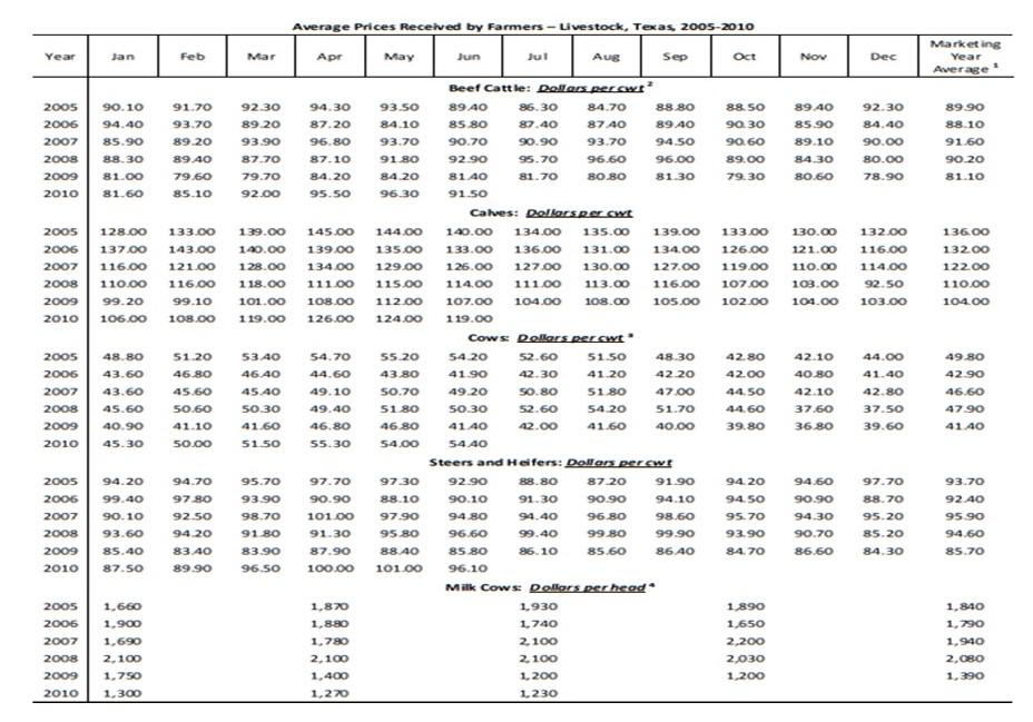
Excel was used to analyze different functional forms that helped determine the trend in cattle production. Regression analysis was adopted for this project due to its predictive nature. Each of the data was checked for accuracy by evaluating the value of R2 and the t-statistics for the regression coefficient for every individual variable. Variables that were statistically insignificant for the current research were dropped. Sensitivity analysis was conducted using the price ratios differences between beef and milk.
Results
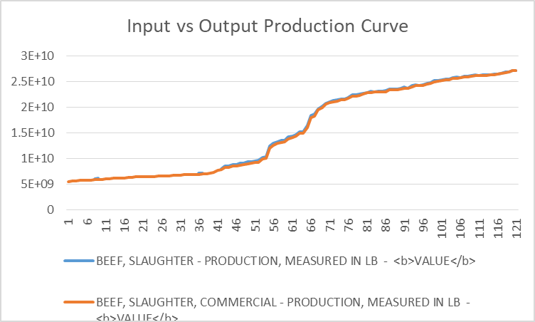
During the analysis of the data, different methods were tried. The regression analysis conducted on beef, in particular, on the production and market costs revealed the output presented in table 2 below. The output indicates a significant relationship between input prices and the associated outputs. Increasing the input prices in beef production increases the rate of production. However, the analysis also reveals that cost increases to a specific limit, after which an additional input does not result in a significant output.
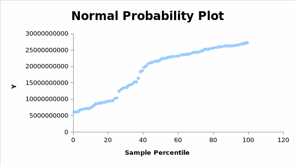
The model indicates that the number of animals slaughtered as the number of beef cattle increased. However, the trend shows a steady rise from 0 to 51, then a sharp rise from 51 to 71, and finally a slow rise. Equating the increase to the cost associated with the input and output variables, and in this case, taking the cost per unit of input and output, based on the definition of equation 1, then it indicates that the optimal price for the input lies at an average of $51 to $71. Consequently, a beef cattle farmer must operate between this particular range to realize a significant output.
In the case for animal feedlot versus sales, there is no statistical significance between the variables.
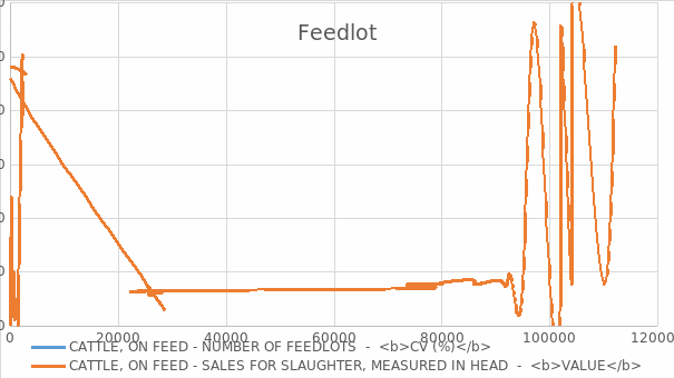
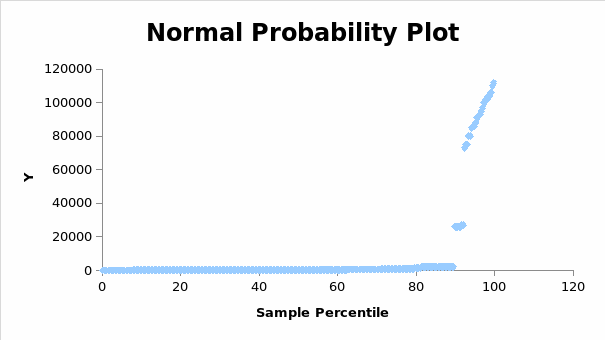
One of the main findings in this project is that the feedlot tends to be quite complicated in determining its direct effect on the cattle products. This is expected because of the different factors that affect animal feed production. In particular, the United States livestock feeds comprise oats, barley, and corn, and all of these are affected by complex factors. An assumption of the annual rainfall of 36 inches may not be sufficient to address the cattle farmers’ needs. In most cases, the production zones have to go to extreme extents of irrigating the farms to have enough food for the cattle.
The data used has indicated that the inputs used in cattle farming may be quite expensive or cheaper, depending on seasons. In particular, the feedlot chart shows seasons when the feedlot rises or falls, revealing the exact nature of the model that can be used to invest in this specific agricultural sector. This particular finding provides farmers with a broader understanding of the impact of different factors on the farm’s output. The model estimates that the regions that experience some specific rainfall patterns, for example, can experience these same trends in production in their farming.
Apart from the effects of rainfall on feedlots, other inputs that affect animal feed production are the ground and fertilizer. Small amounts of feedlot indicate that the farmers did not use a sufficient amount of inputs in raising the crops and grass to help grow the feed. Farmers can find the best feeding materials by incorporating all the necessary inputs to ensure that the cattle can find enough food to cater for all the animals.
The regression analysis indicates that a continuous form of optimal feedlot quantity is significant in realizing maximum output. This shows that the farmers can produce the optimal number of cattle products corresponding to the amount of input they invest in the initial production. However, one thing that is certain about the venture is products always remain higher than the investment. A more significant concern is that exceeding the optimal level of feedstock results in an increase in the marginal cost, thereby lowering the profits. This leaves the question of whether other factors such as medicine and additives can result in losses. This issue is critical because it cannot be assumed that the animals depend only on feedstock. The input and the output have been factored as single variables by assuming that all the inputs combined results in all the output combined. Thus, the results compare the input and the output, thus measuring the entire process’s costs.
In general, these findings indicate that more inputs should be applied in animal feed production to ensure the number and quality of animals produced from the farm and increase profitability. The inputs such as water, veterinary services, and crop production should remain high throughout the year to meet the farms’ demand. However, the producers must also remain sensitive to the seasonal dynamics. The data indicates that the prices and production fluctuate throughout the year. This should point to the fact that farmers should approach the issue in another way, using less input when the seasons or the markets for the animals are low. Such times should be dedicated to raising calves and heifers and release them when the rates begin to be high.
Conclusions and Discussion
The cattle production in Texas impacts the entire economy of the state. As evidenced in the data above, different factors play crucial roles in realizing maximum profits from the operations. However, other multiple factors act contrary to the models adopted; thus, they cannot precisely determine the cattle business trends. In particular, this study majored in understanding the cattle inventory and its impact on production. The analysis has revealed a significant relationship between the two variables. In this case, the higher the inventory, the better production, and profit maximization. This agrees with the model created by Dillon and Heady.
However, other factors such as feedlot do not give a direct link with the production. One of the main reasons for this inconsistency is that feedlot relies on other multiple inputs such as rainfall and fertilizer, and human capital to produce enough food for the cattle. Other inputs, such as labor and cost of medication, are not included in the data, although these play a critical role in determining production. Consequently, farmers need to understand different aspects relating to the amount of feedlot required to make production go up. Most importantly, the model used in this research has revealed that producers with a large number of cattle enjoy the economies of the market, which confirms the reduction in the number of licensed farmers but increased productivity.
References
Dillon, J. L., & Heady, E. O. (1960). Theories of choice in relation to farmer decisions. Iowa Agriculture and Home Economics Experiment Station Research Bulletin, 33(485), 1. Web.
Fox, J., & Weisberg, S. (2018). Visualizing fit and lack of fit in complex regression models with predictor effect plots and partial residuals. Journal of Statistical Software, 87(9), 1-27.
Gardner, G. E. (2019). The economic evaluation of input use prescription maps: Are you paying to make less profit? [Thesis, University of Nebraska-Lincoln]. Digital Commons
Higgins, M. G., Fitzsimons, C., McClure, M. C., McKenna, C., Conroy, S., Kenny, D. A., McGee, M., Waters, S. M., & Morris, D. W. (2018). GWAS and eQTL analysis identifies a SNP associated with both residual feed intake and GFRA2 expression in beef cattle. Scientific Reports, 8, 14301.
Jones, J. W., Antle, J. M., Basso, B., Boote, K. J., Conant, R. T., Foster, I., Godfray, H. C. J., Herrero, M., Howitt, R. E., Janssen, S., & Keating, B. A. (2017). Brief history of agricultural systems modeling. Agricultural Systems, 155, 240-254.
NASS. (2020).Statistics. Web.
Rotz, C. A., Asem-Hiablie, S., Place, S., & Thoma, G. (2019). Environmental footprints of beef cattle production in the United States. Agricultural Systems, 169, 1-13.
Sannikova, M. O., Providonova, N. V., & Sharonova, E. V. (2020). The influence of technical efficiency and weather risk on crop production in Russian agriculture. MS&E, 753(7), 072023.
United States Government Accountability Office. (2020). Science & tech spotlight: Deepfakes. Web.
USDA. (2020a). Cattle and Beef. Web.
USDA. (2020b). Dairy. Web.