Costs
In order to make a business profitable, one must maximize revenues and minimize costs. Maximizing profits does not necessarily mean making great profits. A business should make profits that would make it competitive in the market. At times, reducing the losses a business incurs might be likened to a profit.
Profits are made when the total revenue is greater than both the total variable costs and the total fixed costs. When output is considered in the equation, then the averages of these variables are considered. Therefore, it is also correct to say that profit equals the difference between the average revenue and the sum of the average variable costs and the average fixed costs.
Since the total fixed costs are not affected by changes in the output, it is a constant. Therefore, businesses must try to make the difference between average revenue and average variable costs the greatest. However, it is not straightforward since the average revenue (AR) and average variable costs change with changes in the output. Businesses should find the level of output that would lead to maximum profits or lowest losses.
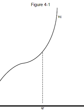
In order to understand this, one must understand the impacts of output on the costs and revenues. An illustration of a short-run total cost curve can be used to understand this. As indicated in Fig. 4-1, the curve touches the y-axis (total cost) at a point representing the business’s total fixed cost. As the name suggests, these costs are fixed and may not be avoided.
These costs may include those incurred during payment of mortgages, security and maintenance. Other costs are further incurred during the operation of the business. However, these costs are not fixed since they vary. They may include those incurred during the purchase of raw materials and those required for labour (work force). Therefore, total costs increase with increase in output.
The technology and equipment that a company has determines the level of output it can produce comfortably and effectively. This level of output has been indicated as Q’ in Fig 4-1. Therefore, a company producing less output than that particular level would imply that it is using its facility to produce less than it can actually produce.
A business can also produce outputs greater than that level of output. However, this would imply that it would incur extra costs to attain that level of output. The choice on whether to operate below or above that level of output (Q’) is dependent upon the demand of the business’s products.
Average Total Costs (ATC)
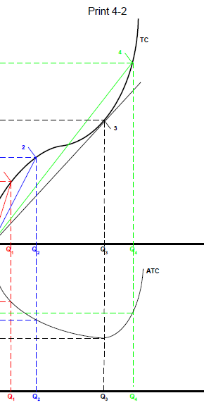
For every business, the average total cost is represented by a U-shaped curve as shown in Figure 4-2. Every amount of average total cost on the curve corresponds to the total cost divided by the output (quantity) produced at that point. Up to some point, the average total cost decreases as the level of output increases. This is evident in the figure since the gradient of the curve decreases as you go along the curve.
The lowest average total cost that a business can incur is at the point of the curve where the line extending from the origin forms a tangent to the curve. This point corresponds to the point Q’ that represents the point at which a business can effectively produce output while using its technology and facilities. Beyond this point, the gradient of the lines drawn from the origin to that point will be progressively increasing along the curve.
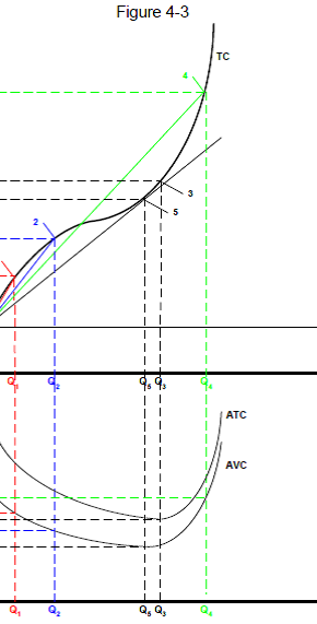
Average variable cost – This value is the difference between TC and TFC. The curve representing the average variable cost (AVC) appears below the ATC and assumes the same shape. The lowest level of AVC is at the point Q5 as shown in Figure 4-3.
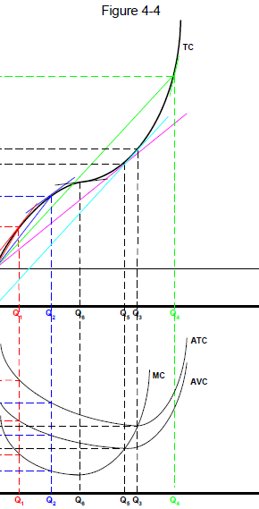
Marginal cost – this is the amount of increase in total cost with every increase in a unit of output. It is represented by the gradient of the TC curve. As shown in the curve of Figure 4-4, the marginal cost is relatively high with small value of output (Q). However, it decreases up to a minimum point then rises again steadily.
Short-run Cost Curves – the ATC, AVC and MC curves lie in such a way as to produce five set of values as related to the quantity produced.
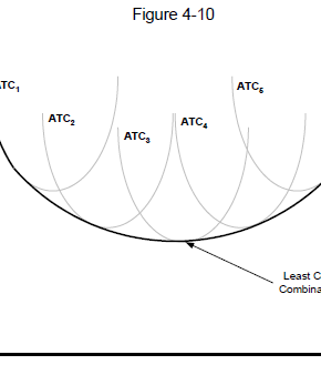
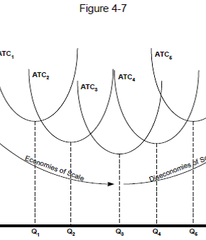
Long-run Average Costs – businesses can use different types of technologies to produce certain amounts of output. For a business to enjoy economies of scale, its ATC curves should progressively become lower at the graph as shown in Figure 4-7. As the levels of operations increase, so does the costs (administrative). Therefore, the ATC curve would start drifting upwards. This way, the business would incur diseconomies of scale. Figure 4-10 shows the smooth long-run average total cost. The lowest point of this curve is referred to as the Least Cost Combination.
Productive Efficiency – this is experienced if the average total cost of running a business is decreasing. This may occur in three different ways. One may be through decreasing the average costs in such a way as not to alter the output or technology and facility used. Secondly, the company may also do this by producing maximum output that the existing facility can handle. Thirdly, the business may move to a facility that would incur less cost.
Demand and Revenues
An indifference curve shows the specific combinations of two products of which the consumer is indifferent. At any point in the curve, the consumer does not prefer any good to the other. Therefore, each point represents a form of satisfaction for the individual. A decrease in the amount of one good would imply that the consumer would need more of the other good in order to be satisfied. Indifference mapping is done to represent indifference curves for various utility levels.
A combination that has a greater quantity of both goods would always yield greater satisfaction to the consumer. This implies that when the indifference curve is shifted upwards, any point in the curve would represent a higher level of satisfaction than the previous. However, budget constraint may limit the consumer’s ability to shift up to another indifference curve.
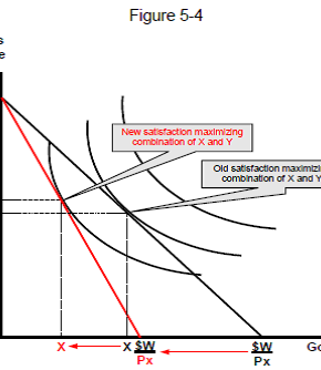
Therefore, the total cost of the combination of both goods must be equal to the customer’s disposable income. At that particular level of utility, a consumer may comfortably substitute one good for the other. If the price of one commodity increases, the budget constraint would shift downwards as indicated in Figure 5-4. The demand for inferior goods usually goes in the opposite direction to that of price.
Price elasticity of demand
This is a measure of the response in terms of demand of the amount of goods or services to the changes in their prices. It represents the percentage change of quantity of the good over the percentage change of its price. When the quantity of the product demanded increases, the price falls.
On the other hand, when the prices fall, the demand of the products increases. Demand is said to be price elastic if the percentage change in quantity demanded is more that the percentage change in price. However, it would be price inelastic if the percentage change in price were greater. When these two variables are equal, demand is unit price elastic.
Total revenue
The total revenue is the product of the quantity demanded and the price per unit. When the demand of a particular good is elastic, increase in its price would reduce the total revenue. The revenue would increase with the decrease in price. However, the case is opposite when the demand is inelastic. Changes in price are proportional to changes in total revenue. When the demand is unit price elastic, the total revenue is the greatest. However, the greatest revenues do not necessarily mean that the profits are also maximized.
Marginal Revenue
Normally, similar goods are sold for the same price per unit. This is what is referred to as uniform pricing. However, other situations demand that the producer sells a particular product at different unit prices or sells the product in different quantities. When it comes to uniform pricing, the price of each commodity is also its average revenue.
Producers are required to know the highest amount of uniform price that he is able to sell his commodities. In order to know this, they require consulting the demand curve. For a producer to sell all his products, he must sell at a particular price per unit. The demand curve also acts as the producer’s average revenue curve.
Other Elasticities
The demand for goods may also be affected by external factors such as competition from similar businesses or fuel prices. Therefore, the changes in the unit price of different commodities (external) may cause a percentage change in the demand of the products. This is what is referred to as the cross price elasticity of demand. If this value is a number greater than or equal to one, then the two different products are substitutes.
A decrease in price of one of the commodities implies an increase in the price of the other. However, if the value is a number below one, then the products are complements. Other elasticities include the income elasticity of demand, which relates to changes in incomes and the price elasticity of supply, which relates to the changes in supplies.
Analysis of a Firm with a Horizontal Demand Curve
In the short run
Firms with a horizontal demand curve are those whose demand curve is perfectly price elastic. This is to mean that the price of the commodities would not be altered whatsoever despite the changes in the supply. Therefore, the marginal revenue of the business is equal to the specified price of the commodity. Likewise, the average revenue of the business would be equal to that of the unit price.
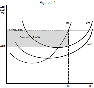
In a graph, the line of the marginal revenue (MR) appears as a straight line. When combined with the curve representing marginal cost (MC), the economic profit that is made by the firm can be determined. All the units produced by the business from zero to the point where a vertical line touches MC at MR, would generate economic profits.
The region where economic profits are obtained is represented by the difference in vertical distance between MR and ATC, as indicated in Figure 6-1. This region consists of maximized profits. However, beyond the point where the curve meets MC, every output would imply greater marginal costs and less marginal revenues. This means that the extra units would only minimize the profits gained by the business.
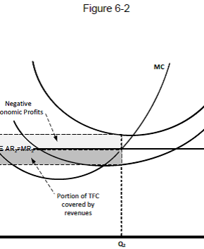
In a case whereby the price (which is equal to the marginal and average revenue of the firm) is placed at a level lower than the line of average total cost (ATC), as shown in the Figure 6-2, every sale of a particular quantity of output would earn negative economic profits. The price set for the commodity would be less than the average cost of producing the product.
This only means that the revenue acquired would not attain the acceptable levels and may at times actually imply that the firm is counting losses. It is at point Q2 in the graph that the company would be experiencing minimal losses. At such a point where the unit price is less than the average variable cost, the business is better off closing down the business than supplying the commodities to the market.
In other occasions, the price set by the market may fall low for other businesses in such a way as to generate revenues too low to meet all the firm’s variable costs. In addition to this, the business would not be able to pay up its fixed costs. The business would be getting losses and the amount of loss would be equal all the fixed and variable costs incurred by the business.
In the long run
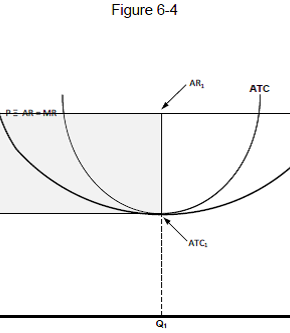
If a business considering a facility that would yield maximum profits builds and operates the plant at a total cost represented by the curve ATC in Figure 6-4, it would be most productively efficient and would produce high average economic profits if it produces quantities of output represented by Q. However, this would not necessarily imply that the firm is also making maximum profits since profit maximization requires the marginal revenue to be equal to the marginal cost.
Therefore, the firm would need to increase its output to a point where MR exceeds MC. The firm can make more profits by ensuring that it operates its business while ensuring that the MR is equal to MC and that the ATC is equal to LRARC at the particular level of output.
At such a position, the firm is very attractive to the clients and this may attract new proprietors who would increase competition. However, it would require many new firms to enter the market and alter supply in order to alter the price. When there are no barriers to entry of suppliers, this might eventually increase pressure and cause reduced prices. New businesses would enter the market for as long as the economic profits are greater than zero. Beyond this point, entry would cease.
At a particular point at the profit-maximizing level of output, the price, AR, MR, MC, ATC and LRATC would all be equal. At this point, the consumers would be enjoying the lowest prices and the businesses would remain functional. When the whole society is put into context, it should ensure that peak productive efficiency and peak allocative efficiency are achieved.
This position is achieved when the price is equal to marginal cost. In this case, when the price is greater than the marginal cost, that would imply an under production. On the other hand, over production would be the case if the marginal cost were greater than the price.
Figures
