Introduction
Investment in real estate is one of the most efficient ways to receive a stable income. One of the most efficient ways to make profitable investments in real estate is to measure price elasticity depending on different variables. The present report utilizes the dataset provided by Anglin and Gencay (1996) to determine house price elasticity using various regression models. The purpose of the paper is to determine the most accurate method for predicting house prices and making judgments about the most appropriate investments.
Simple Regression Model
First, it was decided to create a simple regression model to understand a correlation between the lot size and the price. A standard regression model has the following format: Pi = c+dQi, where:
- Pi is the sale price of a house i in Canadian dollars.
- Qi is the lot size of a house i. in square feet.
The c parameter is an intersect with the y-axis, which is the lowest possible price (assuming the lot size can be 0 square feet). Even though the price can virtually be negative, it is expected that the intersect will represent a minimal price that includes service fees. The d parameter is expected to be positive, as, with the increase of the lot size, the price of the house is to grow. The regression equation is to be interpreted as a demand equation, as it demonstrates how much buyers are willing to pay for houses of different sizes (William and Khim, 2020). The regression line is visualized in Figure 1 below.

The simple linear regression equation is presented below: Pi=34.136 +6.6 *Qi
All the parameters were statistically significant with p<0.001. The adjusted R2 was 0.28, which implies that the model could explain 28% of fluctuations of the price using lot sizes.
Elasticity
The simple linear regression equation presented in Section 1 can be used to calculate elasticity. Elasticity is a ratio that measures the sensitivity of one variable to changes in another. According to Hayes (2020), “most commonly, this sensitivity is the change in price relative to changes in other factors” (para. 1). In econometrics, elasticity is often measured to determine a price policy (Hayes, 2020). If the ratio is below 1, the price is known to be inelastic, which means that changes in a variable mildly affect the price.
There are two types of elasticity, which are arc and point elasticities. Arc elasticity is measured over an arc of the demand curve, which is very useful for real situations, as price changes occur in jumps (Nipun, 2020). Arc elasticity yields only approximate measures, as it virtually connects two price points on the arc with a straight line. Point elasticity measures elasticity at a particular point. The arc elasticity will be more applicable to the present regression model.
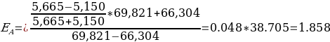
For example, assuming that the size of a house is 5,150 square feet, its price according to the regression model will be: Pi=34.136 +6.6 *5.150=68.126 CAD
If the size of the house increased by 10% (5,150 * 1.1 = 5,665 square feet), the price will also grow by 10%: Pi=34.136 +6.6 *5.665=71.525 CAD
Then, arc elasticity will be the following:
Point elasticity will be calculated as follows:
Logarithms
After transforming the variables of the model presented in Section 1 in logarithms, the predictability of the equation improved with adjusted R2=0.335. The scatterplot for the new model is presented in Figure 2 below:

The logarithmic regression model was the following:
The elasticity of price to the lot size would be calculated the following way:
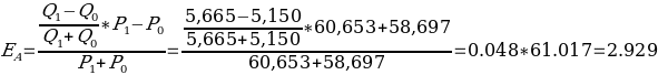
Po = 66.304
Po = 69.821
Optimal Lot size of a House
Knowing the formula for determining a price, a builder can calculate an optimal lot size for a house. The optimal lot size is determined by the profit maximization rule. In order to maximize the profit, marginal profit should be equal to marginal cost. Since there are no fixed costs, the marginal cost of building a house is calculated using the formula: MC=Q²
The marginal revenue is calculated using the regression model introduced in Section 1, which is the following: MR = 34.136+6.6*Qi
The optimal lot size will be calculated as follows:
Q² = 34.136 +6.6 *Q
Q² – 6.6 Q – 34.136 = 0
Therefore, the optimal lot size for a house is 188 square feet.
Multiple Linear Regression
The estimations made for simple linear regression presented in Section 1 were far from being reliable, as the model could explain only 28% of fluctuations of the price. However, the results could be improved by adding more independent variables and using multiple linear regression to make a comprehensive model. We decided to include the following variables into the analysis:
Pi The sale price of house i in Canadian dollars, Qi
The lot size of a house i. in square feet, Pri
The house located in the preferred neighbourhood of the city? Gi
The number of garage places, Ai
Does the house have central air conditioning? Gasi
Does the house use gas for hot water heating? Bedi
The number of bedrooms, Bathi
The number of full bathrooms, Si
The number of stories excluding the basement.
The regression model was estimated as follows:
All the variables of the model reached statistical significance (p<0.001) of alpha=0.05, except for the intercept (p=0.649). The number of bedrooms almost reached statistical significance with p=0.056. The model had the highest predictive ability among the models introduced in Section 1 and Section 3, with adjusted R2=0.64. This implies that the equation can explain 64% of fluctuations in the price of the houses.
The equation can be explained the following way. With an increase of the lot size of a house by one square foot, the price increases by $3.8. The price increases by $12,037, if the house is situated in a preferred neighbourhood. With every garage place, the price of a house increases by $4,534. If the house has central air conditioning, its price goes up by $13,419. If the house uses gas to heat the water, its price increases by $13,047. Every bedroom adds $2,038 to the price, while every bathroom is associated with a price increase of $15,124. Finally, the price goes up by $5,983 with every storey.
Estimations Using the Multiple Regression Model
Assuming that all the continuous dependent variables are at their mean values, and the houses do not have central air conditioning, gas for heating water, and are not located in a preferred area, the price of the house will be:
If we increase the lot size by 10%, the price will be the following:
Hence, arc elasticity of price to lot size will be:
If added a garage place, the price will be:
This is a 7.72% change in the price of the house.
If added a storey, the price will be:
This is a 10.19% increase in price.
Estimations
The provided multiple linear regression model can be utilized using to make various estimations. For instance, the model can be used to estimate the amount that customers are willing to pay for a one-storeyed house of 1,000 square feet with two bedrooms, one bathroom, without gas for hot water heating, air conditioning, or place of a garage, which is not in a preferred area. The estimated price will be the following:
The model can also be used to decide which is the best way to increase its price. In order to decide, which is the best investment, return on investment (ROI) needs to be calculated.
Assuming the cost of adding a bathroom is $3,000:
Assuming the cost of adding a bedroom is $1,000:
Assuming the cost of installing gas for hot water is $2,000:
Assuming the cost of installing central air conditioning is $2,000:
Assuming that it costs $4,000 to make a garage:
Considering these calculations, the most efficient way to invest $5,000 will be to install central air conditioning and gas for hot water as well as adding a bedroom. By making such changes, the price of the house will increase by $28,504.
Further Considerations
If the purpose of the analysis is to estimate the impact of public investment on the house price in a specific neighbourhood of a given city, a longitudinal study needs to be done. The researchers would need to measure the average prices of the houses and amount of public investment in iterations every month or quarter. The measurements then will be analyzed using a linear regression model, which is used to understand the correlations between dependent and independent variables (Tanner, 2016). The dependent variable will be the average price of houses, and the independent variable will be the amount of money invested by the government. The results of such research are likely to be biased, as public investments are likely to lead to gentrification (Zuk et al., 2018). Therefore, the study will need to include control variables, similar to the ones presented in Section 5 (Helmenstine, 2020). Even though such research will have high reliability, longitudinal studies are difficult and costly to perform (Cherry, 2019). Therefore, researchers may want to think of a cross-sectional alternative.
Conclusion
The results of the analysis revealed that the most appropriate way to predict house prices is to use a multiple linear regression model that describes a dependent variable using eight independent variables. The equation was useful for calculating the susceptibility of house prices to changes in lot size. At the same time, the equation was useful for choosing the most profitable investments.
References
Anglin, P.M. and R. Gencay (1996) “Semiparametric estimation of a hedonic price function”, Journal of Applied Econometrics, 11(6), pp. 633-648.
Cherry, K. (2019) The pros and cons of longitudinal research. Web.
Hayes, A. (2020) Elasticity. Web.
Helmenstine, A.M. (2020) The role of a controlled variable in an experiment. Web.
Nipun, S. (2020) Difference between arc elasticity and point elasticity. Web.
Tanner, D. (2016). Statistics for the Behavioral & social sciences (2nd ed.). Bridgepoint Education.
Williams, C. and J. Khim (2020) Supply and demand. Web.
Zuk, M. et al. (2018). Gentrification, displacement, and the role of public investment. Journal of Planning Literature, 33(1), pp. 31-44.