Median sale price for houses
The graph below will show the trend of median sale prices for the houses for from 1993 to 2012. The data is presented in quarters.

From the graph above, it is evident that there is an upward trend of median sale prices in all the cities. The trend is upward from year to year in all the quarters. It is an indication of increasing prices of housing over the years. The growth can be attributed partly to increase in the inflation level and partly to increase in the level of economic activity in the regions. Inflation increased from 65.7 in the first quarter of review 104.5 in the last quarter (Rabinowitz 2004)
Estimation of the mean
The graph below shows the trend of the mean value of sale prices.
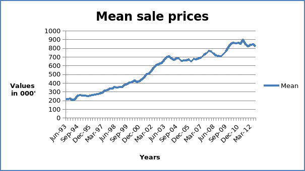
The mean value of sale prices was increasing over time. It is shown by the upward trend of values over time. This could be an indication of the structural increase in the long run and the equilibrium. This could also be as a result of an increase in interest rates. Increase in interest rates increases the cost housing thus increasing the sale price of houses.
Simple linear time regression
Regression analysis is a statistical tool that is used to develop and approximate linear relationships among various variables. Regression analysis formulates an association between several variables. When coming up with the model, it is necessary to separate between dependent and independent variables.
Regression models are used to predict trends of future variables. The section carries out a simple linear regression between the mean sale price of houses and time. The mean sale price will be the explained variable while the explanatory variable will be time (Arnott & McMillen 2006)
The regression line will take the form Y = b0 + b1X
Y = Mean prices
X = Time
The theoretical expectations are b0 can take any value and b1 > 0.
Regression Results
The table below summarizes the results of the regression.
From the above table, the regression equation can be written as Y = -74738.9 + 37.59659 X. The intercept value is not dependent on the area of the house but on other factors such as the location of the house. The value captures all other factors that were not included when modelling the regression line. The coefficient value 37.59569 implies there is a positive relationship between mean sale price and time. The value of the coefficient of determination is high and it shows a strong positive relationship between the two variables.
Real median prices
Converting the nominal median sale prices to real median sale prices eliminates the effect of inflation. The real values are arrived at by using base year as a reference point and taking into account the consumer price index.
Once the effect of inflation has been eliminated, one can now evaluate the real change in the median sale prices. From the calculations done, the real values are lower than the nominal values of median sale prices. However, the mean values still has the same trend as those for nominal median values as shown in the graph below.
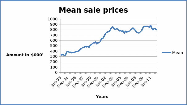
The graph above shows that there is an increase in the values for real sale prices over time. The results of the regression line are shown below.
The regression line will take the form Y = b0 + b1X
Y = Mean prices (real)
X = Time
The theoretical expectations are b0 can take any value and b1 > 0.
Regression Results
The table below summarizes the results of the regression.
From the above table, the regression equation can be written as Y = -59995.3 + 30.27972 X. The intercept value is not dependent on the area of the house but on other factors such as the location of the house. The value captures all other factors that were not included when modelling the regression line.
The coefficient value 30.27972 implies there is a positive relationship between mean sale price and time. The value of the coefficient of determination declined from 95.50% to 86%. The value is still high and it shows a strong positive relationship between the two variables.
The growth in real sale prices between September 1993 and September 2003 is 157.08% while the growth between December 2003 and September 2012 is (7.16%). It can be deduced that there was a rapid growth in real sale prices between 1993 and 2003 thereafter the prices increased at a declining rate and thereafter started to decline. (Evans 2008). This could be an indication that the government is putting up measures to ensure that there are no serious fluctuations in the sale prices of houses every year (Edwards 2007).
Rent
The growth in real rent between September 1993 and September 2003 is 88% while the growth between December 2003 and September 2012 is 120%. It can be deduced that there was a rapid growth in real rent between Dec 2003 and 2012. The growth rate for the first nine years was 88%. Thus, it can be deduced that there is a general increase in the rent level in Sydney and its regions. The ratio of house prices to income increased over the period. In 1993, the ratio was 0.00883 in 1993.
The value increased to 0.010211 in 2012. This can be attributed to an increase in rent over the years. There was an increase in the rental yield over the years. The rental yield in 1993 was 74.78%. The value declined to bout 43% in 2003 thereafter it started to raise. The rental yield in 2012 was 81.43%. The graph below shows the relationship between rental yield and the ratio of house prices to income (O’Sullivan 2011; O’Sullivan & Gibb 2008)

The graph above shows that there is a negative relationship between rental yield and the ratio of house prices and rent. This can be seen in the downward trend that can be seen in the points in the diagram above. Prices and rent series tend to move in the same direction (McMillen & McDonald 2011; Arnott & McMillen 2006).
Explaining the relative movement of prices
There has been rapid growth in the property prices in the regions. The growth between 1993 and 2003 was more rapid than the growth rate between 2003 and 2012. This can be attributed to government interventions to stabilize the price of housing (Riley 2009).
References
Arnold, R 2011, Economics, Cengage Learning, USA.
Arnott, R & McMillen, D 2006, A companion to urban economics, Blackwell Publishing Ltd., USA.
Edwards, M 2007, Regional and urban economics and economic development: Theory and methods, Auerbach Publications, New Delhi.
Evans, A 2008, Economics and land use planning, John Wiley & Sons USA.
Mankiw, G 2011, Principles of economics, Cengage Learning, USA.
McMillen, D & McDonald, J 2011, Urban economics and real estate: Theory and policy, Hamilton Printing Company, USA.
O’Sullivan, A & Gibb, K 2008, Housing economics and public policy, John Wiley & Sons USA.
O’Sullivan, A 2011, Urban economics, McGraw-Hill Education, USA.
Rabinowitz, A 2004, Urban economics and land use in America: The transformation of cities in the twentieth century, M.E. Sharpe, USA.
Riley, G 2009, Housing market economics digital textbook, Tutor2u Limited, USA.