Econometrics. Portfolio Strategy: Equity and Commodity Market Research Paper

Introduction

During the recent recession, there has been an increased tendency among buyers to sell their stock options and invest in commodities like oil, metals, agricultural products, etc. investors had started demanding more of copper and crude oil as the buyers diversified from bonds (Carpenter, 6 November 2009). Analysts had predicted this as a trend to remain for some time as they believed that investors were allured by the stability of prices of commodities like gold and oil (Carpenter, 6 November 2009). According to the S&P GSCI Index, 24 commodities rose by 46 percent in 2009, after a 43 percent drop hit it in 2008 due to global recession and drying up of raw material demand (Carpenter, 6 November 2009). The reason, many states, is due to the interests that many investors have shown in the commodity market as a means of diversifying their portfolio. Another argument for this is that the devaluation of the US dollar has helped in holding up the commodity prices (Pressman, 10 January 2008). Thus, analysts predict that the US dollar’s devaluation against the euro will increase the prices of commodities further (Carpenter, 6 November 2009). However, the question remains, under these circumstances whether, commodity prices can maintain their upward movement or will the recessionary pressure bring down the commodity prices.

The recent shift in the preference of investors from equity to commodities brings up the question that is commodity less volatile than equity. Further, there arises a need to assess the future risk, price, and volatility of both commodities and equity to assess the composition of the future portfolio.

Research in economics and business has historically tried to predict the future risk and volatility of stock markets. The ability to forecast financial volatility using an econometric model has been researched by many academicians and there are many models dedicated to this purpose. In this paper, the risk and volatility of both the equity and commodity market will be assessed using the historical data from S&P500 and GSCI indices. The analysis of risk and volatility is done using the GARCH model (Engle, 2001).

Literature Review

The commodity is an excellent portfolio diversifier. Proponents who believe that commodities are a suitable alternative for stock or bond investors believe that it is a lucrative form of diversification (Greer, 2000; Miffre & Rallis, 2007). Greer (2000) argues that recently there has been an increase in diversification of portfolio into commodities and the reason behind the trend is comparable volume and volatility as in equity. Further, the returns from commodities have shown a more positive skew historically, which has led to its recent popularity (Greer, 2000). Therefore, Greer studied data from 1970 until 2000 and found that risk and returns from the commodity index show more positive total returns as compared to the equity index. Greer also finds that the commodity index is negatively related to the bond and equity index and that it is positively correlated with inflation and changes in inflation (2000, p.50). Therefore, this finding indicates that commodities provide excellent immunity against inflation.

Another study was conducted by Gorton & Rouwenhorst (2006) to study the characteristics of commodity futures as an asset investment using the equally weighted index of commodity futures and their monthly returns between 1959 and 2004. Their study demonstrates that commodities futures have provided the same returns as Sharp ratios for the period. The risk premium of commodity futures is found to be the same as that of equities, however, the commodity returns are found to be negative as that of equity. They also find that commodity prices have a positive relationship with inflation, unexpected inflation, and changes in expected inflation (Gorton & Rouwenhorst, 2006).

Miffre & Rallis (2007) studied the occurrence of short-term prolongation and reversal in long term in the commodity market. They identify 13 profitable momentum strategies that are expected to generate a 9.38 percent average return annually. When they analyzed these commodities on a long-term basis they found that “The momentum returns are also found to have low correlations with the returns of traditional asset classes, making, therefore, our relative-strength portfolios good candidates for inclusion in well-diversified portfolios.” (Miffre & Rallis, 2007, p.1886)

Thus, research on the commodity as an asset provides evidence –both empirical and theoretical – that commodities are a lucrative option for a diversified portfolio and when inflations are expected to be high.

Methodology

GARCH Model

Research to measure the volatility of the equity market has been extensively done. There are various models, which are there which are utilized for understanding the future expected volatility of prices and attached risk. This section deals with the understanding of the previous researches conducted, and the expected results from the same. Bollerslev (2001) provided a summary of the various econometric financial models that have been developed over the past three decades. In his essay, he indicates that there developed time-varying models of volatility as in ARCH, stochastic volatility models, and robust movement-based procedures like GMM (Bollerslev, 2001, p.42). Previous research has documented the reason for large (small) price changes will be followed by other large (small) changes (Fama, 1965), however, it was Engle (Engle, 2001) and Bollerslev (1986) studied the time-varying model of volatility. Using GARCH various empirical research has been done and volatility, spillovers, linkages, variances, and correlations has been found (Bollerslev, 2001). This model has been consistently been used for forecasting “continuous-time stochastic volatility” (Bollerslev, 2001, p.43). Therefore the validity of the model is empirically tested by many scholars (Bollerslev, 2001). For this research, GARCH is used for studying and furcating daily data of equity and commodity indices. The next section provides the theoretical background of the model.

The Model

Here a brief description of the theoretical model of GARCH (Bollerslev, 1986) is presented. Taking I_t to be the stock market index, and r_t its returns, we can construct the following equation as r_t = log I_t – log I_t-1. For this research, the t denotes daily observations in changes in equity and commodity indices. Even though there are higher order models for future predictions are useful, the most popular model in use to determine r_t is the autoregression of order p with GARCH(1,1). The disturbances are therefore found to be (AR(p) – GARCH (1,1)), which can be expressed as:

• Φ_p(B) r_{t =} µ + Ɛ_t, with Φ_p(B) = 1 – Φ₁B – … – Φ₁B^p
• Ɛ_t ~ N(0,h_t)
• h_t = ω + αƐ²_t-1 + βh_t-1

Here B is defined as the backward shift operator shown algebraically as B^kx_t = x_t-k. the parameter µ is a constant which in reality is estimated to be a value very close to or equal to zero (Franses & Dijk, 1996). Further, α and β are polynomials of order p and q here taken to be 1. Further, the value of p is usually zero or less, implying that that there are no options to forecast r_t from its past historical data. Further, Bollerslev (1986) takes the following assumptions – (i) Φ(z) = 0 and lie outside the unit circle, (ii) Ω, α, β >0, and (iii) α+β<1.

The odd moments of Ɛ_t in the model (1) are equal to zero and therefore Ɛ_t and r_t provide a symmetric time series with a fat tail (Bollerslev, 1986; Franses & Dijk, 1996). The r_t for stock markets may show negative skewness which is internally built as stock markets are expected to crash more quickly and frequently as opposed to boom conditions, and that the absolute magnitude of the crashes are much larger than the booms (Franses & Dijk, 1996, p.230).

Data

The above-described model is used to analyse the volatility of the stock and commodity indices from the period 1 January 2008 to 31 March 2010. Historical data is collected for daily stock and commodity price indices (Yahoo! Finance, 2010). The stock index that is used is S&P500 and the commodity index used for the study is GSCI.

The first observed date is 1 January 2008 and the last observed date is 31 March 2010. Figure 1 presents the plot for the daily closing rates of the indices. S&P500 is measured in primary axis indicated by the red line and GSCI is plotted on the secondary axis represented in blue. The diagram shows that in early 2008, when the global recession had begun to set in, the prices of the stock index was falling, while that of the commodity index was rising. However, after the seventh month they started following similar trend of rise and fall.

Table 1 shows the descriptive statistics of the returns of the closing prices of the two indices. The total number of observations for both the indices is 565 for both the indices. The mean and the variance are relatively small (Franses & Dijk, 1996). The kurtosis of the series if more than 0 indicating that fat tail distributions describe the variables under study. The skewness is positive in both the indices implying that the distribution of the indices have a long right tail. The Jarqua-Bera series is used to test is the series is normally distributed. At 5% level, the Jarqua-Bera test rejects normality.

The main purpose of the research is to predict the volatility of the two indices and to identify which is a better strategy of portfolio allocation, GARCH model is used to analyse the reasonable large data sample from 2008 to 2010. Thus, we choose daily samples for little more than a year that indicates the recent recessionary time-period.

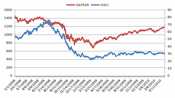
Table 1: Summary statistics of data on returns, Source: Yahoo! Finance

Data Analysis and Discussion

In table 2, the GARCH model is reported for S&P500 and GSCI indices. Here GARCH (1, 1) model is used (see equation 1) to estimate the volatility of the time series data as this model is enough to capture any volatility in data (Brooks, 2008). The values of α, β, and ω are shown in table 2. The conditional variances of both the indices are changing, and the conditional variance is a constant 0.2. Further the sum of α and β is close to but less than 1.

Log likelihood is computed from the product of all the conditional densities of the standard errors of the given primary data. For S&P500 data convergence was achieved after 6 iterations and for GSCI it was achieved after 33 iterations. This implies it took 6 iterations to maximize the likelihood function and standard errors in case of Bollerslev-Wooldridge following Engle (2001). The three coefficients in the variance equation are listed as ω, the intercept. The other two coefficients are α and β that signifies the first lag of the squared sum and the latter represents the first lag of the conditional variance. The analyses reverts a mean variance process as α and β sum up to be less than 1. As the sum is very close to one, the process is expected to revert very slowly (Engle, 2001). Z-statistics provide the standard error i.e. the ratio of the coefficients and standard error, and the probability value are also provided in the table. Table 2 also provides a 15 period lagged Lung-Box test that will help in finding the autocorrelation. The autocorrelation using Lung-Box test for S&P500 gives a coefficient of 0.06, which is not large rather it is significant. Lung-Box test for GSCI is 375.3071 and it has a probability of 0. The positive value indicates that it is not a common indicator in most economic time series data as has also been observed by Engel (2001). However, it holds serious implications for GARCH model. As the probability is zero therefore it shows that the model does not have ARCH, which is consistent with the findings off Engle (2001).

Then the standard deviation of the portfolios and its one percent quartile is forecasted in table 3 for both S&P500 and GSCI. This is done for the period from 1 January 2008 to 31 December 2009.

In order to evaluate the true volatility of GARCH, it is necessary to forecast the time series properly. As is mostly done in case of forecasting volatility (Franses & Dijk, 1996), w_t is measured which is defined as:

• w_t = (r_t – r^–)²

Here ris the average over last 25 days of daily observations. Therefore, the predictions are observable in table 3. The predictions are plotted in figure 2. The predicted value of S&P500 is expected to increase initially then stat falling from mid of January 2010. In February, there is a further dip in hate stock market and then it starts rising by end of February 2010. GSCI index has been following similar trend in 2010, with only showing minor rise in end of January 2010. However, it started falling by end of February 2010. Figure 2 and 3 presents the GARCH volatility for the indices S&P500 and GSCI for 1 January 2008 through 31 March 2010 of S&P500 and GSCI indices from 2008 to 2010. Figure 2 show that the equity index is expected to be as volatile as the GSCI index. On the contrary, commodity index is expected to fall more than the equity index as it takes a downward plunge in January 2010. Further, the GARCH volatility demonstrated in the figure shows that both the indices co-vary in the same direction. Thus, the indices follow a similar volatility pattern.

Table 2: GARCH Estimates

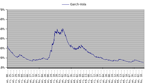
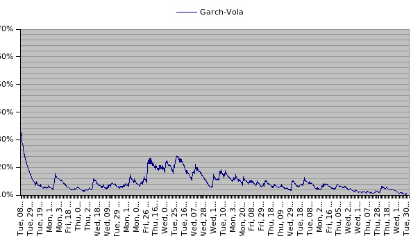
GARCH volatility demonstrated in figure 2 and 3 for S&P500 and GSCI indices indicates that the S&P500 is less volatile than GSCI as the α + β are less than 1 but are very close to 1 in case of S&P500, whereas in case of GSCI, it is less than 1, but are less closer to 1. The estimate for log likelihood for S&P500 is 1485.61 and the GARCH volume is plotted in figure 2. The log likelihood for GSCI is -1509.25 and its GARCH volatility is plotted in figure 3. The figure shows that S&P500 index shows more volatility in the period under study than GSCI index. The maximum volatility for S&P500 index was reached 50% in July 2008 and then it started to fall. 50% volatility indicates that the stock index was 50% chance of going up or down. Then there was a fall in volatility indicating that the stock index was gaining back its stability. GSCI volatility plotted in figure 3 shows that the volatility of the prices in commodity market is very low. The volatility ratio is close to 10% and the maximum was reached in January 2008 when it was 30%. Therefore, it can be concluded that equity market is more volatile than stock market. Therefore, the strategy adopted by investors during the recession was correct as the risk volatility in the commodity market, from the above analysis, is found to be much less than that of equity market.

Figure 4 and 5 shows the graph with the predictions done using GARCH (1, 1) model. The predictions shows that the equity market index is expected to become more volatile in 2010. The expected volatility in the equity market will increase and the volatility in the commodity market is expected to remain stable from January through August 2010. Therefore, the future predictions for commodity shows that it is expected to give less volatile returns and prices are expected to fluctuate less as compared to equity market.

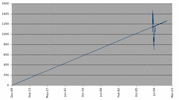
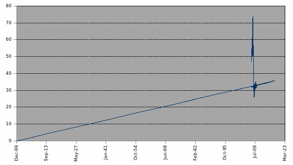
This indicates that the risk associated in investing in equity in future is expected to be higher than in commodity market. Thus, future assessment of risk and price volatility of the equity and commodity market indicates that commodity market has lesser volatility than equity market. Further, the predicted prices of equity market are expected to rise in future, while that of commodity prices are expected to remain more or less stable at one point with minor movements. This observation implies that the investment into the equity market in late 2009 would have fetched more profit for the investors as there is an expected rise in prices in future. In case of commodity market there will be rise in gains, however, the change is very stable and low indicating less gain.

Conclusion

The main question that the research wanted to answer is that if the latest trend in increase in investment in commodity a better option during the recession than equity. The study conducted on the daily equity index of S&P500 and daily commodity index of GSCI was analysed for volatility using GARCH model. The commodity index showed less volatility than the equity index. The equity index has more risk associated than commodity. Further, the future predictions of the equity index shows that in the future the prices are expected to rise and in the future while that of commodity prices are expected to remain stable with minor changes. These findings are in accordance to previous studies done on commodities (Gorton & Rouwenhorst, 2006; Miffre & Rallis, 2007). From this finding two conclusions regarding portfolio decision can be made:

1. Commodity is a better form of investment when there is a recession as commodity index has been found to have a positive correlation with inflation, and when the equity prices are going down due to recession, commodity prices remain less volatile. Therefore, investment in commodity is a better option if the investor aims to make a less risky portfolio. Therefore, investing is commodities can be considered to be a ‘good’ in case of recession.
2. A balanced combination of equity and commodity is a good portfolio option, as the former being more risky, gives higher returns, and the latter is less volatile and has less changes in prices, and therefore gives lesser returns. However, the latter gives immunity to external shocks of the market to the portfolio allocation, thereby, reducing risk.

Reference

Bollerslev, T., 1986. Generalized autoregressive conditional heteroskedasticity.. Journal of Econometrics, 31, pp.307-27.

Bollerslev, T., 2001. Financial econometrics: Past developments and future challenges. Journal of Econometrics, 100, pp.41-51.

Brooks, C., 2008. Introductory econometrics for finance. 2nd ed. Cambridge, UK: Cambridge University Press.

Carpenter, C., 2009. Commodities Demand Is ‘Trend to Stay,’ Barclays Says. Web.

Engle, R., 2001. GARCH 101: The Use of ARCH/GARCH Models in Applied Econometrics. Journal of Economic Perspectives, 15(4), p.157–168.

Fama, E.F., 1965. The Behavior of Stock-Market Prices. The Journal of Business, 38(1), pp.34-105.

Franses, P.H. & Dijk, D.V., 1996. Forecasting Stock Market Volatility Using (Non-Linear) Garch Models. Journal of Forecasting, 15, pp.229-35.

Gorton, G. & Rouwenhorst, K., 2006. Facts and fantasies about commodity futures. Financial Analysts Journal, 62(2), pp.47-68.

Greer, R.J., 2000. The Nature of Commodity Index Returns. The Journal of Alternative Investments, 3(1), pp.45-52.

Miffre, J. & Rallis, G., 2007. Momentum strategies in commodity futures markets. Journal of Banking & Finance, 31(6), pp.1863-86.

Pressman, A., 2008. Commodities: Boom or Gloom? Web.

Yahoo! Finance, 2010. Yahoo! Finance. Web.