Free market and mixed economy
An economic system is made up of the organizations and the techniques that are used to determine the commodities to be produced, the approach of producing them, and the intended consumer of these commodities. These decisions are important because resources are scarce. There are several types of economic systems. In this paper, the free market and mixed economy will be discussed. The two economic systems have different characteristics. In the case of a free-market economy, resources are allocated by the forces of demand and supply. Thus, either an individual or a group of central players cannot allocate resources. In a free-market economy, the price mechanism ensures that all aspects of the economy are in balance (Douma & Hein 2013).
For instance, growth in demand pushes the price upwards. This stimulates manufacturers to increase production. Further, the amount of consumption depends on the income of individuals. Therefore, in a free-market economy, a government will concentrate on safeguarding property rights (Tucker 2010). A free-market economy is hypothetical and does not exist in the real world. In the case of a mixed economy, resources are owned by both the public and the private sector. A mixed economy can also be viewed as a market economy with significant government involvement. In most cases, a government intercedes to rectify market failures and to provide public and merit commodities. Most economies in the world are mixed (Ruth & Hannon, 2012).
A change in quantity supplied and change in supply
There is a difference between a change in supply and a change in quantity supplied. The differences are explained below.
A change in quantity supplied
A change in quantity supplied can be explained as the movement long a stationary supply curve while holding other factors constant. This movement is drawn from the law of supply, which states that there is a positive relationship between price and supply while holding other factors constant (Perloff 2012). Thus, if the price moves up along the y-axis, the quantity supplied will move to the right along the x-axis. A change in quantity supplied is caused by price movements. This relationship is shown in the graph below.
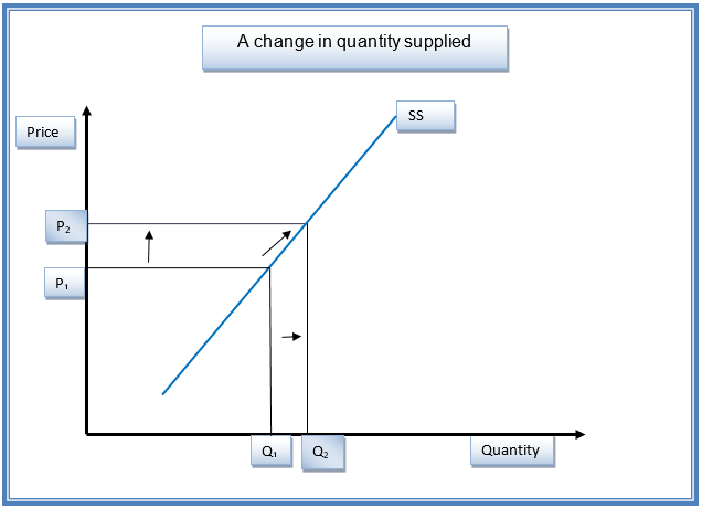
An increase in price from P1 to P2 will cause an upward movement on the supply curve, as shown by the arrow. This will cause the quantity supplied to increase from Q1 to Q2 (Adil 2006).
Change in supply
Change in supply is caused by non-price factors that influence the quantity supplied. These factors can make the supply curve to shift to the right (an increase) or to the left (a decrease). Some of the non-price factors are increases in the number of suppliers, change in technology, subsidies, and a decline in the price of raw materials, among others. A change in supply can be illustrated using a graph, as shown below (Parkin 2007).
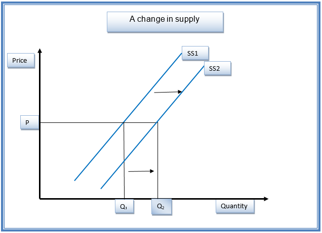
In the graph above, favorable non-price determinants will cause the supply curve to shift from SS1 to SS2. This makes the quantity supplied to increase from Q1 to Q2. It can be noted that the price does not change. An opposite movement occurs if unfavorable non-price determinants are experienced (Bade & Parkin 2013).
Cross price elasticity of demand
This type of elasticity measures the degree by which a change in the price of one commodity affects the change in demand for another commodity. In arithmetic terms, it is the percentage change in quantity demanded of one commodity, Y, divided by the percentage change in the price of one commodity, X. The resulting coefficient of elasticity shows how sensitive the demand for one commodity is to the changes in the price of another commodity. Examples of two substitutes are butter and margarine (McEachem 2008).
These two cannot be consumed at the same time. Therefore, if the price of butter rises, by the law of demand, the quantity demanded will fall. Further, consumers will prefer to consume more of the substitute, which is margarine. In the case of substitutes, when the price of one commodity increases, then the quantity demanded of the best alternative, that is, the substitute increases. In this case, the value of the cross-price elasticity is positive. Complementary goods are consumed together (Moon, 2013).
Examples of two complementary goods are rice and chicken. If the price of chicken goes up, then by the law of demand, its quantity demanded will drop. Since rice complements chicken, then its quantity demanded rice will also drop. Based on the analysis above, if the cross-price elasticity is zero, then it implies that the two commodities being analyzed are not related (Barber 2010). Further, if the value of elasticity for the commodities is less than one (negative), then it indicates that the two products are complementaries. Finally, if the elasticity is greater than zero (positive), then it shows that the two commodities being analyzed are substitutes. In the United States, the cross elasticity between cantaloupe and watermelon is 0.6. This shows that they are substitutes. Further, the cross-price elasticity between chicken and rice is -0.1309. This implies that they are complementaries (Jain, 2006). Thus, the study of cross-price elasticity helps in monitoring market trends.
Income effect and substitution effect
Based on the law of demand, a change in price can be described in terms of income and substitution effect. The diagram presented below will be used to explain these effects.
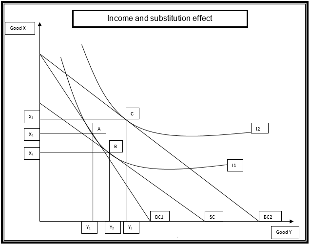
The two items that will be analyzed are commodity Y and X. According to the law of demand, a drop in the price of commodity Y will lead to an increase in quantity demand. The increase will cause the budget line to pivot from BC1 to BC2. Also, the indifference curve will shift from I1 to I2. This represents a movement to a higher indifference curve. The equilibrium position is the point of tangency between the budget line and the indifference curve (Tucker 2012).
When the price of commodity Y falls, a consumer will be indifferent between consumption at point A and B because they lie on the same indifference curve. However, at point B, the consumer shall not have exploited the budget. A fall in price increases the quantity of commodity Y that can be consumed as represented by budget line BC2. This shows that real income has grown as a result of a drop in price. Thus, the consumer can increase consumption to point C on a higher indifference curve I2 from point B on a lower indifference curve (Baumol & Blinder 2011). At this point, an individual will consume Y3 and X3 of commodity Y and X, respectively.
Thus, the movement from Y2 to Y3 is due to the income effect. The change from point A to B is known as the substitution effect. This can be attributed to the fact that the individual will reduce consumption of X, from X1 to X2, and increase the use of commodity Y, from Y1 to Y2. It can be observed that this occurs on the same indifference curve I1 (McEachern 2011). It implies that the consumer is substituting Y with X. The total effect is the sum of income and substitution effect, that is, the sum of the movement from Y1 to Y2 (substitution effect) and change from Y2 to Y3 (income effect).
Perfect competition and monopoly
Perfect competition and monopoly are considered to be the extreme forms of market structures. These two have distinctive features. Some of the features are discussed below.
Number of firms
There are several firms that operate in a perfectly competitive industry is made up of a large number of small firms. These firms are price takers. Besides, no single firm can have market control. Under monopoly, there is only a single firm that has market control. Moreover, it determines the price in the market (Mankiw 2012).
Availability of substitutes
Under perfect completion, the commodities are homogenous, and there is an infinite number of products. In the case of a monopoly, there is only one commodity with no close substitute (Arnold 2008).
Entry and exit
Under perfect competition, there is free entry and exit of firms. Barriers do not exist. In the case of a monopoly, there is a barrier to entry.
Information
In the case of perfect competition, information concerning the production methods and prices is readily available and known by all players. This information is not readily available in the case of a monopoly (Anderton 2008).
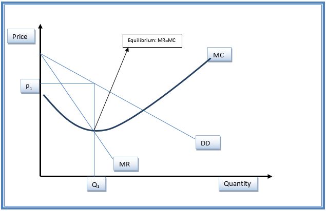
These unique characteristics create differences in the shape of the revenue and cost curves (Baldwin & Scott 2013). The graphs presented below show the equilibrium position of the two market structures.
Perfect competition
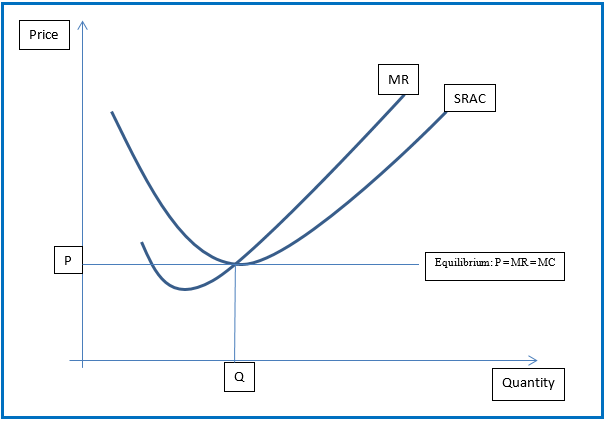
Monopoly
References
Adil, J 2006, Supply and demand, Capstone Press, USA. Web.
Anderton, A 2008, Economics, Pearson Education Inc., UK. Web.
Arnold, R 2008, Economics, South-Western Cengage Learning, USA. Web.
Bade, R & Parkin, M 2013, Essential foundations of economics, Pearson Education Inc., USA. Web.
Baldwin, W & Scott, J 2013, Market structure and technological change, Taylor & Francis Publishers, UK. Web.
Barber, R 2010, Elasticity, University of Michigan, New York. Web.
Baumol, W & Blinder, A 2011, Economics: principles & policy, Cengage Learning, USA. Web.
Douma, S & Hein, S 2013, Economic approaches to organizations, Pearson Education Inc., London. Web.
Jain, T 2006, Microeconomics and basic mathematics, V.K Publications,New Delhi. Web.
Mankiw, G 2012, Principles of microeconomics, South-Western Cengage Learning, USA. Web.
McEachem, W 2008, Microeconomics: a contemporary introduction, Cengage Learning, USA. Web.
McEachern, W 2011, Economics: a contemporary introduction, Cengage Learnings, USA. Web.
Moon, M 2013, Demand and supply integration: The key to world-class demand forecasting, Pearson Education Inc., USA. Web.
Parkin, M 2007, Economics, University of Michigan, USA. Web.
Perloff, J 2012, Microeconomics, Pearson Education Inc., England. Web.
Ruth, M & Hannon, B 2012, Modelling economic systems, Springer Science & Business Media, USA. Web.
Tucker, I 2012, Macroeconoics for today, Cengage Learning, USA. Web.
Tucker, I 2010, Survey of economics, Cengage Learning, USA. Web.