Commodity Markets: Customers Rule
Generally, consumers dictate market dynamics, example, if consumer demand is high, the market will respond by increasing supply and vice versa. The market response process entails six fundamental stages. To understand the market response dynamics, market-level diagrams have to be constructed. Figure 1 and 2 demonstrates how individual demand curves and supply curves can be used to derive a market demand curve and market supply curves respectively. The two figures show that when more buyers and suppliers enter into the market, the market demand and supply curve shifts. Decrease in demand or supply will shift the aggregate demand or supply curve on the opposite direction.
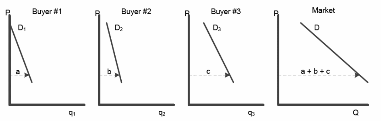
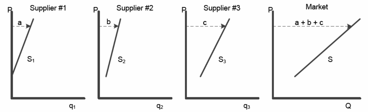
The three individual supply curves are the portion of the suppliers’ marginal cost curve that lies above their average variable cost curve. In the real commodity market, the number of suppliers and buyers are very many. For this reason, the market demand and supply curves are highly compressed.
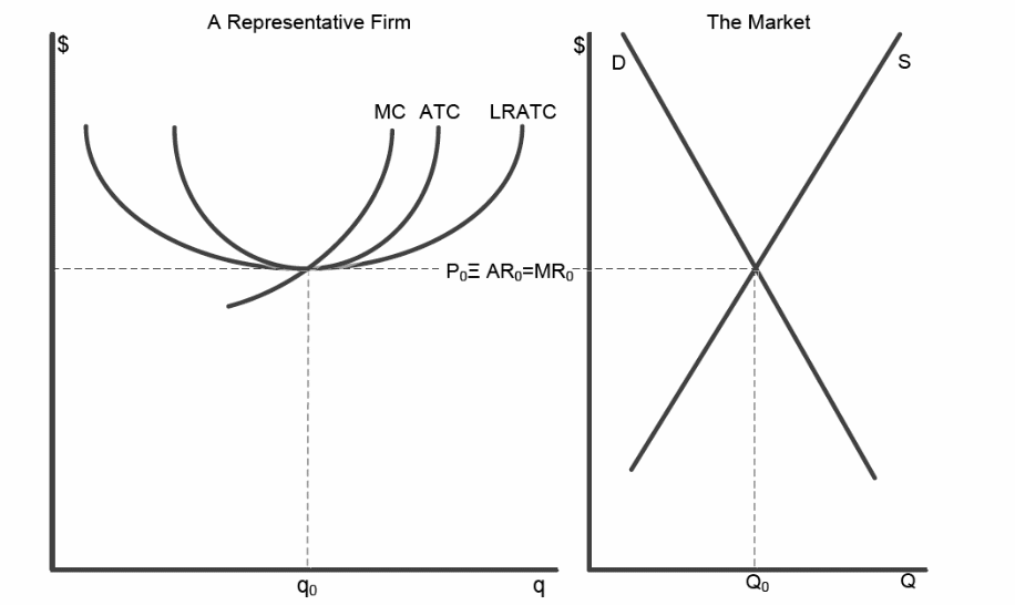
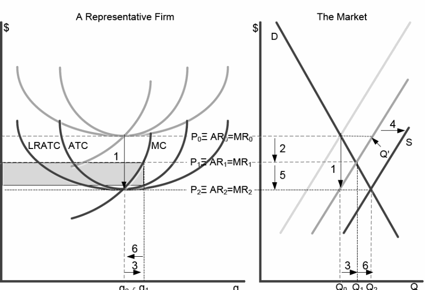
Figure 3 shows the cost structure of a representative supplier and the market equilibrium. The long-term market equilibrium satisfies three conditions, that is, demand and supply equals, the suppliers are maximizing their profits, and the profits made by the suppliers are enough to guarantee their sustainability. It is important to note that at the long-run equilibrium P=AR-MR=MC=ATC=LRATC.
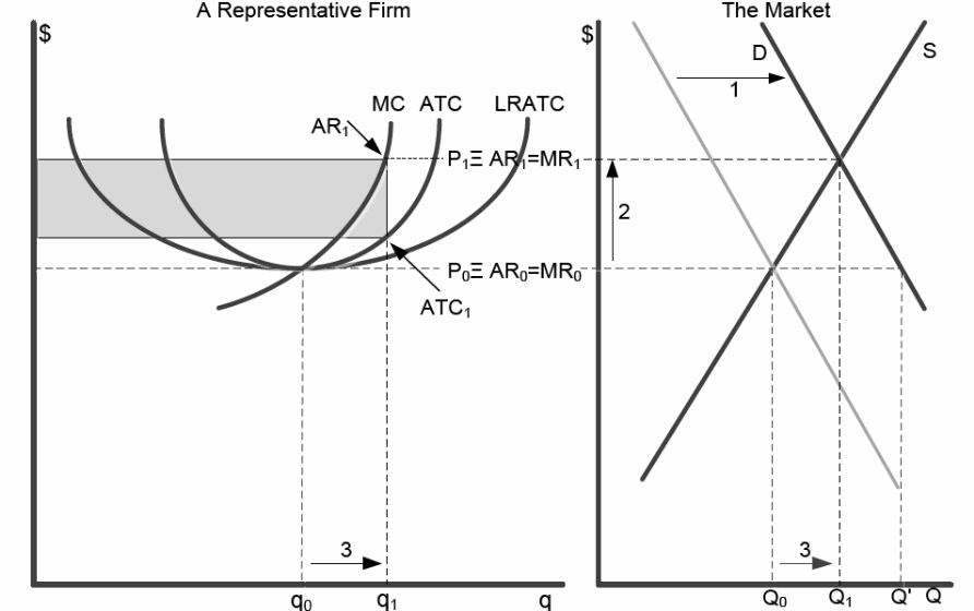
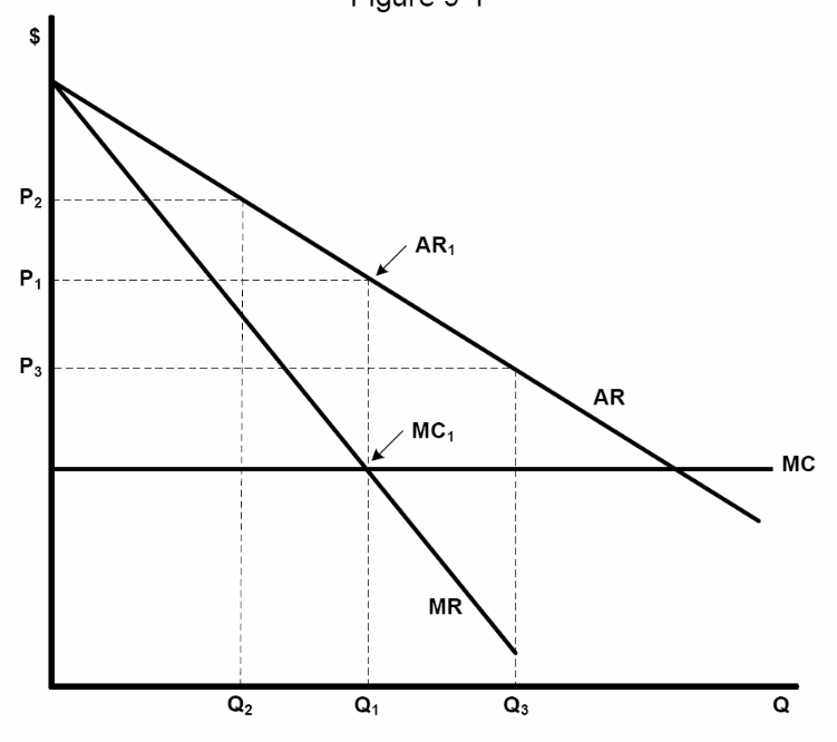
An increase in commodity demand shifts the market demand to the right as shown in figure 4. This represents the first step. Q’ units of the product will be available at the prevailing price. Since demand is positively correlated with price, the suppliers will increase their price to p1 in order to equate the new demand and supply. As the price increases, a number of buyers will react by reducing their demand (Q’ to Q1). This represents the second step.
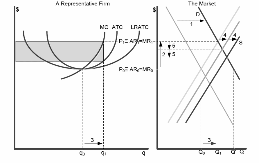
At the same time, suppliers will increase supply along the individual marginal cost curve and as a group along the aggregate supply curve. The increase in supply is due to the fact that individual suppliers normally maximize profit when they operate on their marginal cost curve at the prevailing price level. Suppliers cannot increase supply without increasing prices. Increase in supply without price increment means the marginal cost will surpass marginal revenue for the entire product. This is the reality of the individual supplier’s cost structure. This marks step 3. The shaded area represents the economic profit made by the supplier. The profit normally attracts new entrants and this will shift the supply curve to the right as shown in figure 5. This represents step 4. As the number of the new entrants increases, the existing suppliers will be forced to lower their prices to arouse demand and, in so doing, link supply to demand. This represents step 5.
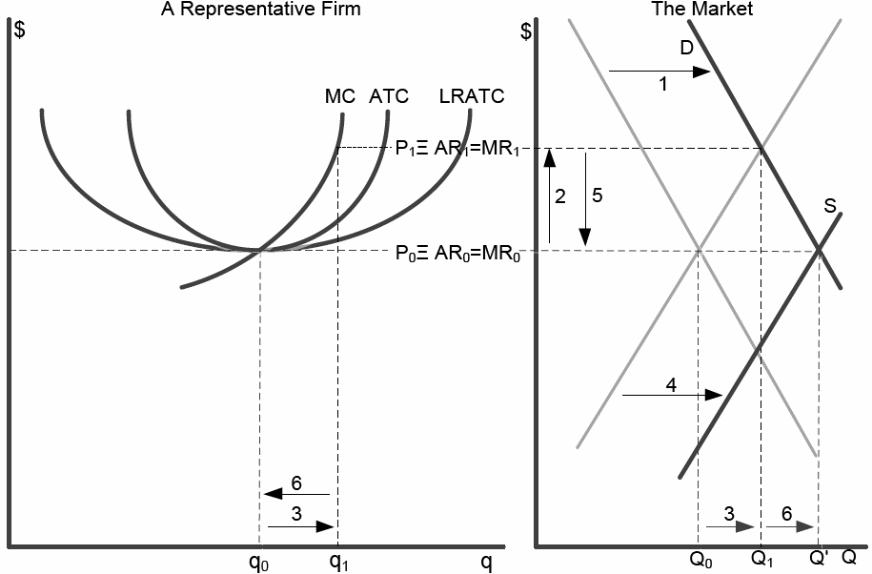
The entry of new suppliers will go on as long as the market is profitable. However, the profit will shrink due to the falling prices. The suppliers will respond by lowering the marginal cost curve so as to avoid making losses. This is well illustrated in figure 6 and represents step 6.
Entries and exits may leave the long-run equilibrium with zero economic profit. This means the market cannot withstand any increase in costs. Therefore, the cost has to be passed to the consumers. Figure 7 shows what happens when the marginal cost curve rise because of increased cost. Any rise in cost curves is matched by a rise in the aggregate supply curve.
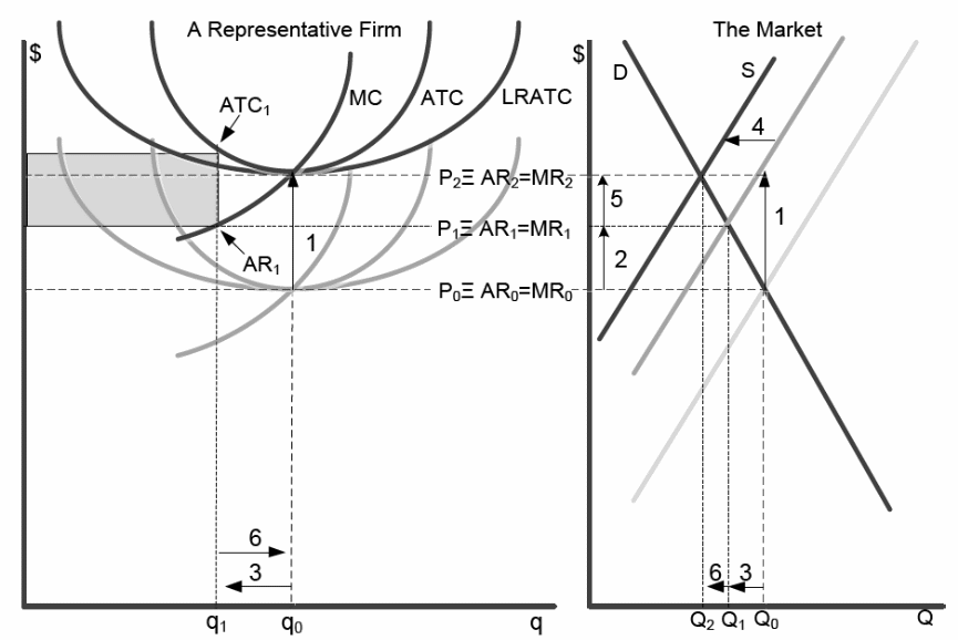
At the prevailing price P0, increase in cost prompts suppliers to reduce output. They attempt to do away with all the units whose marginal cost exceeds marginal revenue. If the prices were to remain the same, the volumes will fall to quantity Q’. However, as the quantity falls, the suppliers are forced to increase prices to P1 to equate supply and demand. Since the demand curve is slopping, the price increase is higher than the cost. The firm reduces supplies from q0 to q1 to minimize losses. At q1 the marginal cost is at the high price level. This means the high cost is passed to the consumers, but that is not good enough because of the negative economic profit. The negative economic profit will force some firms out of the business. However, the negative economic profit will only persists until many suppliers have exited the industry. The exit reduces supply and, therefore, prices increase to P2.
The drop in the cost structure is matched by a corresponding drop in the aggregate supply curve. At the prevailing price PO, supply will increase as long as the marginal revenue is above the marginal cost. If the prices were to remain the same, supply will increase to Q’. However, additional increases in price will force the price down to P1 to equate demand and supply. As the prices go down, the firms reduce supply from q1 to q0. This ensures that firms operate on the marginal cost curve at the prevailing price level. An additional supply from the new entrants is able to offset the reduction in supply.
Non-Commodity Markets
In economics, products are commodities with indistinguishable versions. However, products with different versions are referred to as non-commodities. Non-commodity products can be created through product differentiation. Some of the most common non-commodity products include shoes, cars and aircrafts among others. For instance, there are a wide variety of shoes and each has unique characteristics. Non-commodities give consumers unmatched opportunities for commodities that not only suit their pockets, thanks to different product varieties, but also suit their diverse tastes and preferences.
Using product differentiation, a firm can create a market niche and, therefore, can influence the price of its product. However, this does not mean the supplies can totally control both market prices and volumes. What they can do is set prices and let the market determine the volumes and vice versa. All in all, the objective of the suppliers do not change in both commodity and non-commodity market, that is, profit maximization.
By reducing supply, the firm can create an artificial shortage that would push the price up and vice versa, hence the demand curve slopes to the right. However, in the case of many competing commodities, the slope is relatively gentle. An attempt to push prices up would lead to loss of sales to the rivals. On the contrary, few competing products would have a steep demand curve. This is because firms have a considerable power over market niche.
Figure 8 shows a typical scenario of a firm that has created very little demand for its product to guarantee sustainability. The AR line represents the highest price that would be paid for competing products. On the other hand, the LRATC represents the lowest average cost that would be paid for similar competing product. It can be seen that at each level, the AR is exceeded by LRATC. Negative economic profit cannot be avoided in this case. In free market economies, losses are as significant as profits. Normally, losses are as a result of wastefulness. As a result, they can be avoided through efficient use of scarce resources.
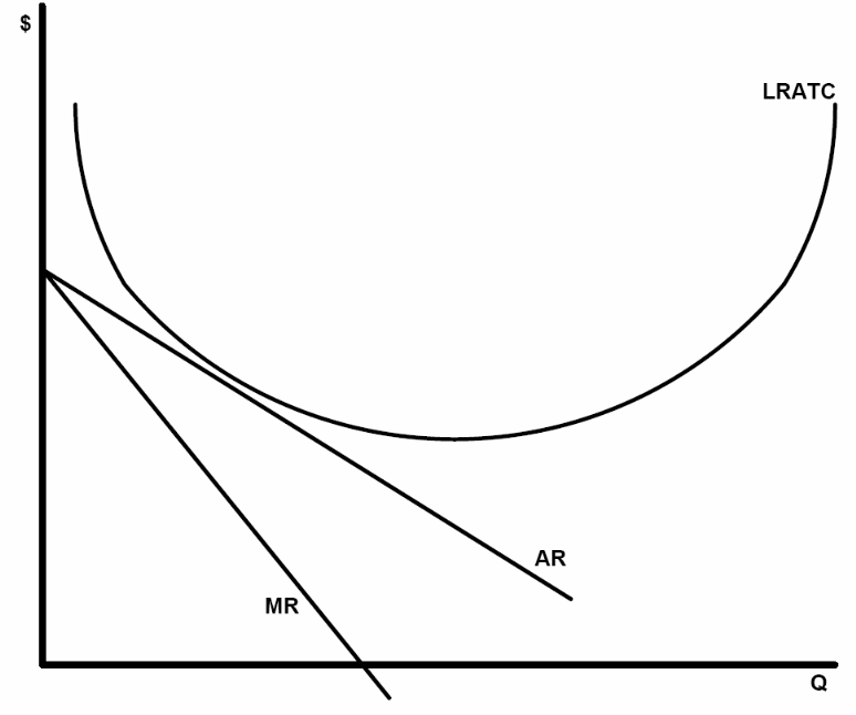
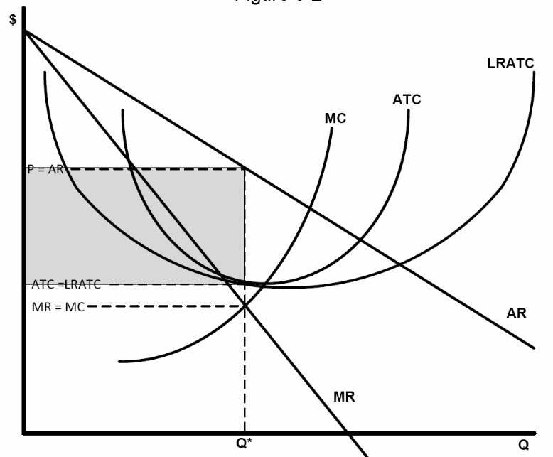
Figure 9 shows an efficient/profitable supplier of a non-commodity. So long as a section of the AR curve lies above the LRATC, there is a possibility of making some profit. Maximum profit is realized where the resource (represented by ATC curve) and the supply (Q*) fulfil two conditions. First, MR=MC. Second, AT= LRATC. The shaded area is the maximum economic profit. Efficiency can also be achieved when the firm operates at the lowest average cost per unit. In other words, the firm is operating at the bottom of the ATC curve. In addition, efficiency can be achieved when the bottom of the ATC curve is at the bottom of the LRATC. In a country where resources are scarce, all the three forms of efficiency are vital. This can be achieved when firms face horizontal demand curve, and this can only take place in commodity markets. Nonetheless, non-commodity market can also achieve efficiency, but they tend to be rather productively inefficient. This implies that they only operate with the first type of efficiency (where MC=MR and ATC= LRATC.
Optimal “allocative efficiency” call for the prevailing price to equal marginal cost (P=MC). However, this cannot be achieved in non-commodity market. Hence, non-commodity firms do not supply socially-optimal volumes and, in so doing, slows down the general standard of living.
Speical topics
Markup Pricing
The profit maximization rule of a firm dictates that MC=MR and the AR must be above the ATC. The firm determines the supply volumes, while the demand determines the price. Markup pricing is a situation where the merchants set the price and let the demand determine the volumes. Figure 10 shows how markup pricing works. The demand is represented by AR and MC represents the present wholesale cost. ATC and LRATC have been left out to minimise overcrowding of diagrams. The supplier will opt for volume Q1 for price P1 (MC=MR). Note that the markup is the perpendicular distance between MC to AR. In other words, the supplier determines the profit maximizing volume, whereas the demand determines the markup.
Where is the demand curve?
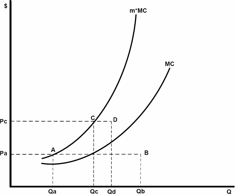
When a new product is being introduced into the market, it is always difficult to determine the product’s demand. The main objective of the firm is profit maximization, but at what volume and price. The firm could engage the services of a marketing research firm, but that would be very expensive. Alternatively, it could experiment using markup factors and sales estimates. Figure 11 shows an example of such experiments. The figure displays two MC curves (mc and m*mc). The perpendicular height of the m*mc equals to the selected markup factor, which is m times the MC at each quantity. With set price and quantity, the firm can experiment until it establishes the profit maximization volume and price.
Price Differentiation
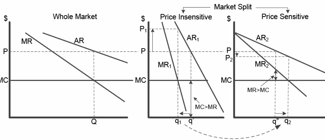
This refers to selling a similar product to different market segments for different prices. The prices tend to be low for price sensitive consumers than price insensitive consumers. The price sensitive consumers are said to have elastic price elasticity of demand. On the other hand, insensitive consumers have inelastic price elasticity of demand. Figure 12 oversees the price differentiation analysis. To make the analysis simple, let’s imagine a firm with a constant marginal cost. The ATC and LRATC have been left out to minimise overcrowding of diagrams. For this reason, there will be no clear hint of profit. Q is the profit maximization volume. For price insensitive buyers, the supplier will increase the price to P1 and, therefore, reduces the quantity from q to q1. For buyers with elastic price elasticity of demand, the prices are reduced to P2, hence the quantity increase from q to q2. The diagram to the left provides the summation of the revenues.
Monopoly
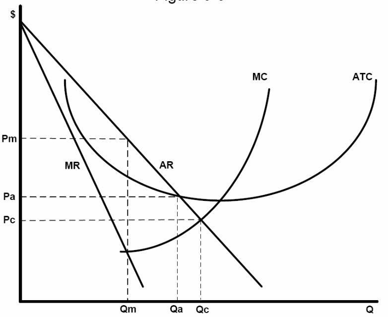
This is a firm whose products have no matching substitute. For that reason, the firm has exclusive control of the market. These kinds of suppliers normally make supernormal profits. Entry to such market is always restricted either by the government policies or by their sheer dominance. Examples of monopolists are government units and large pharmaceutical companies among others. Figure 13 shows the monopolistic characteristic of public utility monopolies.
The monopolists would wish to set supplies at Qm and prices at Pm. However, the state would want it at Qc and Pc in order for the price to equal marginal cost (allocative efficiency). Unfortunately, this will force the price below the ATC (at Pa and Qa). At Pa and Qa, the utility can barely cover its cost.