Missing Values
Strength and weaknesses in using SPSS to analyze missing values
Missing values create a serious problem during analysis. Therefore, the SPSS Missing Value Analysis program tries to solve this problem. However, this program has a number of strengths and weaknesses. The first strength is that the program offers a variety of charts and graphs that facilitate the analysis of missing values. Further, the program can be able to handle complex data set and create new variables from the existing information. It also provides a variety of analyses such as deletion and imputation methods that other programs do not offer. In addition, the program is simple to use and allows for easy management of data (Meyers, Gamst, & Guarino, 2013).
A major drawback of this program is that some of the words that are used in the analysis of missing values are specific to the program. Therefore, it requires prior knowledge in order to use it.
How the data met underlying assumptions of the analysis procedure
Data cleaning
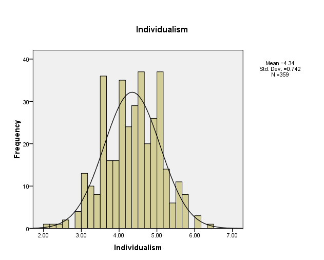
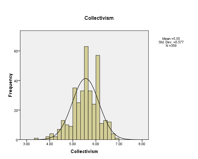
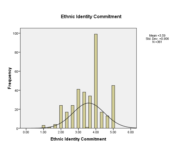
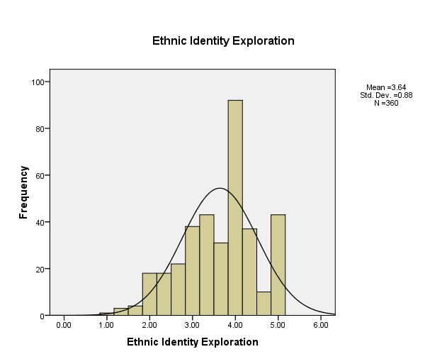
To analyze how the data met the underlying assumptions of the analysis procedure, the process of data cleaning will be carried out. This will be achieved by using descriptive statistics and a histogram. The analysis will be focused on the four continuous variables. The results are presented below.
The descriptive statistics for individualism, collectivism, ethnic identity commitment, and ethnic identity exploration show that skewness and kurtosis are within the normal range. This is also supported by the normal curve that is superimposed on the histograms that are presented below. In addition, the means and the standard deviations of the four continuous variables seem realistic. A further review shows that there are 12 system missing values. From this preliminary assessment, it can be concluded that the data is clean (Wooldridge, 2013). However, there is a need to further analyze the missing values.
Missing values analysis
The descriptive statistics for the missing values is summarized in the table below.
The results show that the number of missing values for continuous variables range between 10 and 12 while the percentage of missing values vary between 2.7% and 3.2%. Thus, it can be noted that the proportion of missing values is less than the threshold of 5%. The mean and standard deviation are also shown in the table above. This will have a significant impact on the choice of technique that will be used to resolve the problem. Further, the results of t-test detect continuous variables that have strange missing value patterns. It tries to show whether respondent with missing data differ from those that do not have missing data. The results of t-test are not statistically significant. The mean difference is small and it is a sign of MCAR. Further, it will be important to analyze the patterns of missing values so as to establish whether the data is mutually missing or individual cases are missing multiple variables. The results of patterns are displayed below.
The first row shows that there 327 cases of no missing values on any of the variables. The second and third rows show that there are 10 cases of missing values for gender and ethnic identity commitment. The fourth subset contains 10 missing values for individualism and collectivism. This can imply that there is a lack of nonrandom in the missing values. Further, fifth subset contains 12 cases of missing values for ethnic identity exploration.
A test for missing completely at random (MCAR) can also be carried out. This will help in determining the strategy that can be used to solve the problem. The results for the Little’s MCAR test are presented in the table below
The results show that the significance is 0.196 and it is greater than the significance level of 0.05. The results are not statistically significant and it shows that the missing values are MCAR. The results indicate that the missing values are not related to other observed values. Thus, list-wise deletion or single imputation procedures can be used to correct the missing value problem.
Solving the missing value problem: list-wise deletion
The selection of list-wise deletion technique is based on the fact that the proportion of missing value is less than 5%. Further, the missing data are MCAR. This method will entail deleting cases with missing values. The results are presented below.
After carrying out list-wise deletion, the sample size will be reduced to 337. However, there will be no significant change in the mean values of the four variables as shown in the table above. The results also show that there will be low percentages of correlation between the variables apart from the case of ethnic identity commitment and ethnic identity exploration.
This technique has a number of limitations. The first limitation is that it can lead to a loss of data that might have been expensive to obtain. It may lead to a reduction of the sample size. This may have an effect of reducing the statistical power and increasing the estimate of measurement error (Verbeek, 2017).
Outliers
Strength and weaknesses in using SPSS to analyze outliers
The main strength of this program is that it offers a variety of methods that can be used to analyze outliers. A major drawback of using SPSS to analyze outliers is that relying on one test may lead to interpreting the data wrongly. For instance, the stem-and-leaf diagram does not show all outliers. Therefore, there is a need to use various tests and tools. Another challenge is that the graphic editor is not flexible. Therefore, adding information on the stem-and-leaf diagram is not possible (Bade & Parkin, 2014).
How the data met underlying assumptions of the analysis procedure
In this case, descriptive statistics, and stem-and-leaf diagram will be used to evaluate whether the data meet the underlying assumptions for the analysis procedure (Gujarati, 2014). The results for descriptive statistics and histogram are discussed in the previous section. The emphasis will be put on the stem-and-leaf diagram.
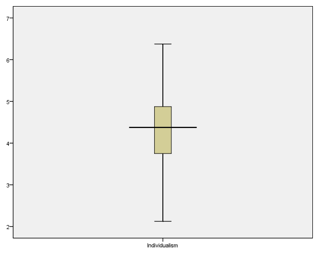
The diagram above for individualism shows that the data is fairly normal. There are no outliers in the data set.
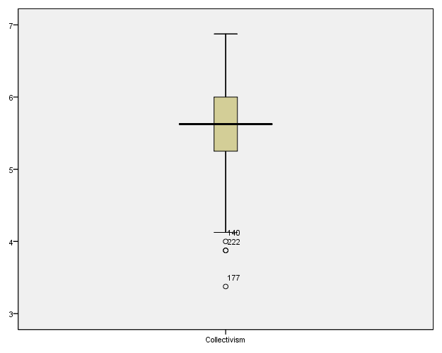
In the case of collectivism, there are three cases of outliers. These are 140, 222, and 177.
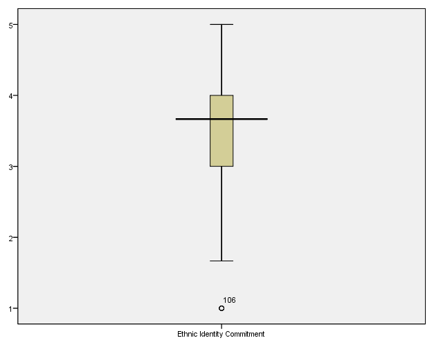
There is only one outlier, that is, case 106 for ethnic identity commitment.
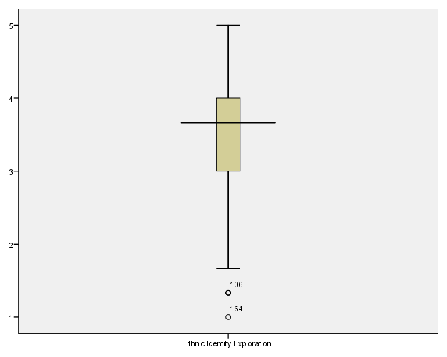
In the data set for ethnic identity exploration, there are two cases of univariate outliers. They occur in cases 106 and 164. It is worth mentioning that the stem-and-leaf diagram does not give complete information on the outliers. For instance, case number 235 occurs for both ethnic identity commitment and ethnic identity exploration. Further, there are other outliers that are not identified in the stem-and-leaf diagram. These case numbers can be found in the attached SPSS output.
A technique that is used to handle outliers
A comparison of the results from the four continuous variables shows that case numbers 106 and 235 occur for both ethnic identity commitment and ethnic identity exploration. Therefore, they should be excluded from further analysis. A major limitation of deleting the outliers is that it can result into missing values which may further complicate the process of analysis. It may also reduce the sample size.
References
Bade, R., & Parkin, M. (2014). Essential foundations of economics (2nd ed.). New York, NY: Pearson Education.
Gujarati, D. (2014). Econometrics by example (2nd ed.). New York, NY: Macmillan Publishers Limited.
Meyers, L. S., Gamst, G. C., & Guarino, A. J. (2013). Performing data analysis using IBM SPSS (6th Ed.). New Jersey, NJ: John Wiley & Sons, Inc.
Verbeek, M. (2017). A guide to modern econometrics (5th ed.). New Jersey, NJ: John Wiley & Sons, Inc.
Wooldridge, J. M. (2013). Introductory econometrics: A modern approach (5th ed.). Mason, OH: South-Cengage Learning.